Evaluating a Calibrator Honestly

Two questions this notebook answers:

1. How do you measure calibration without fooling yourself? Scoring a calibrator on its own training data does not merely flatter it — for an isotonic-family calibrator it reports perfect calibration by construction.

2. When a model gets worse, which part broke? A single score says “worse”. The CORP decomposition says how much is miscalibration you can fix and how much is lost discrimination you cannot.

Both rest on the same machinery: isotonic regression via the pool-adjacent-violators algorithm, which is what calibre is built on throughout.

Reference: Dimitriadis, Gneiting & Jordan (2021), Stable reliability diagrams for probabilistic classifiers, PNAS 118(8).

import matplotlib.pyplot as plt
import numpy as np

from calibre import (
    IsotonicCalibrator,
    confidence_bands,
    consistency_bands,
    corp_reliability,
    cross_val_calibrate,
    debiased_calibration_error,
    score_decomposition,
    sweep_calibration_error,
)
from calibre.metrics import expected_calibration_error

rng = np.random.default_rng(20260731)

1. A reliability diagram with no bins to choose

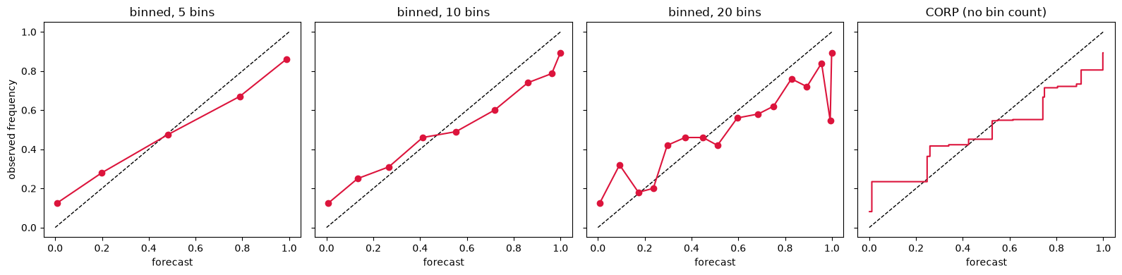
The classic reliability diagram makes you pick a bin count, and the picture changes with the choice. Below, the same forecasts are binned three ways — the apparent calibration swings with the bin count, which is an artifact of the analyst’s choice rather than a property of the model.

CORP removes the choice: isotonic regression decides the number and position of the flat segments, optimally and automatically.

n = 1000
truth = rng.uniform(0, 1, n)
labels = rng.binomial(1, truth).astype(float)
# A mildly overconfident forecaster.
forecasts = np.clip(1.4 * (truth - 0.5) + 0.5, 0.001, 0.999)


def binned_curve(x, y, n_bins):
    edges = np.quantile(x, np.linspace(0, 1, n_bins + 1))
    idx = np.clip(np.digitize(x, edges) - 1, 0, n_bins - 1)
    xs, ys = [], []
    for b in range(n_bins):
        m = idx == b
        if m.sum():
            xs.append(x[m].mean())
            ys.append(y[m].mean())
    return np.array(xs), np.array(ys)


fig, axes = plt.subplots(1, 4, figsize=(16, 4), sharex=True, sharey=True)
for ax, n_bins in zip(axes[:3], (5, 10, 20)):
    xs, ys = binned_curve(forecasts, labels, n_bins)
    ax.plot([0, 1], [0, 1], "k--", lw=1)
    ax.plot(xs, ys, "o-", color="crimson")
    ax.set_title(f"binned, {n_bins} bins")
    ax.set_xlabel("forecast")

diagram = corp_reliability(forecasts, labels)
axes[3].plot([0, 1], [0, 1], "k--", lw=1)
axes[3].step(diagram.x, diagram.cep, color="crimson", where="post")
axes[3].set_title("CORP (no bin count)")
axes[3].set_xlabel("forecast")
axes[0].set_ylabel("observed frequency")
plt.tight_layout()
plt.show()

2. Is the deviation real, or is it noise?

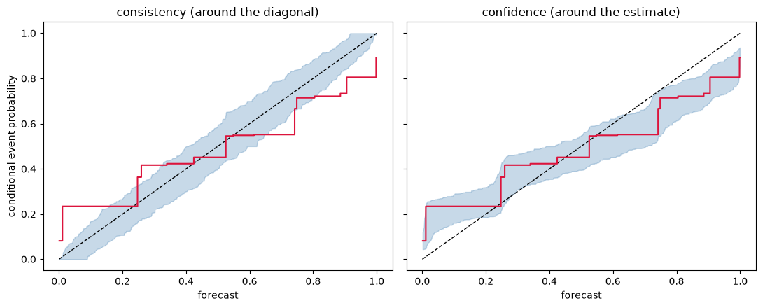
A curve off the diagonal means nothing without knowing how far a calibrated forecaster would stray by chance. Consistency bands answer exactly that: outcomes are redrawn as y* ~ Bernoulli(x) — taking the forecasts at face value — and the diagram refit. The bands sit around the diagonal, and a curve leaving them is the analogue of a small p-value.

Confidence bands answer the other question, clustering around the estimate instead.

band = consistency_bands(forecasts, labels, level=0.9, n_resamples=400, random_state=0)
conf = confidence_bands(forecasts, labels, level=0.9, n_resamples=400, random_state=0)

fig, axes = plt.subplots(1, 2, figsize=(11, 4.5), sharey=True)
for ax, (b, title) in zip(
    axes,
    (
        (band, "consistency (around the diagonal)"),
        (conf, "confidence (around the estimate)"),
    ),
):
    ax.fill_between(b["x"], b["lower"], b["upper"], alpha=0.3, color="steelblue")
    ax.plot([0, 1], [0, 1], "k--", lw=1)
    ax.step(diagram.x, diagram.cep, color="crimson", where="post")
    ax.set_title(title)
    ax.set_xlabel("forecast")
axes[0].set_ylabel("conditional event probability")
plt.tight_layout()
plt.show()

outside = np.mean((diagram.cep < band["lower"]) | (diagram.cep > band["upper"]))
print(f"fraction of the curve outside the 90% consistency band: {outside:.1%}")

fraction of the curve outside the 90% consistency band: 54.9%

3. Where did the score go?

score_decomposition splits any proper score into three parts:

mean_score = MCB - DSC + UNC

• MCB (miscalibration) — what recalibration would save you. Fixable.

• DSC (discrimination) — what your scores buy over always predicting the base rate.

• UNC (uncertainty) — the difficulty of the problem. Nobody can change it.

MCB and DSC are non-negative by construction, and the identity is exact.

variants = {
    "honest": truth,
    "overconfident": np.clip(1.6 * (truth - 0.5) + 0.5, 0, 1),
    "underconfident": 0.5 * (truth - 0.5) + 0.5,
    "noise-added": np.clip(truth + rng.normal(0, 0.15, n), 0, 1),
}

print(f"{'forecaster':16s} {'Brier':>8s} {'MCB':>8s} {'DSC':>8s} {'UNC':>8s}")
for name, x in variants.items():
    d = score_decomposition(x, labels)
    print(
        f"{name:16s} {d['mean_score']:8.4f} {d['MCB']:8.4f} "
        f"{d['DSC']:8.4f} {d['UNC']:8.4f}"
    )

forecaster          Brier      MCB      DSC      UNC
honest             0.1780   0.0060   0.0777   0.2497
overconfident      0.1960   0.0207   0.0743   0.2497
underconfident     0.1926   0.0206   0.0777   0.2497
noise-added        0.1962   0.0083   0.0618   0.2497

Read the table by column, not by row.

UNC is identical everywhere — it depends only on the outcomes, so it is the same problem in every row. The forecasters differ in the other two, and they differ in different ways: a monotone squeeze damages MCB while leaving DSC largely intact, because squeezing preserves the ranking. Adding noise damages DSC, because it destroys ranking information that no recalibration can recover.

That distinction is the practical payoff. A high MCB is a call to recalibrate. A low DSC is a call to build a better model.

4. The trap: never evaluate on the training data

For an isotonic-family calibrator this is not a matter of degree. The calibrator and the CORP diagnostic are the same PAV projection, and PAV is idempotent — so in-sample MCB is exactly zero however badly the model generalises. It cannot detect miscalibration even in principle.

cross_val_calibrate returns out-of-fold probabilities: each one from a model that never saw that observation.

in_sample = IsotonicCalibrator().fit(forecasts, labels).transform(forecasts)
out_of_fold = cross_val_calibrate(IsotonicCalibrator(), forecasts, labels, cv=5)

for name, values in (("in-sample", in_sample), ("out-of-fold", out_of_fold)):
    d = score_decomposition(values, labels)
    print(f"{name:12s} MCB {d['MCB']:.6f}   Brier {d['mean_score']:.4f}")

in-sample    MCB 0.000000   Brier 0.1739
out-of-fold  MCB 0.005128   Brier 0.1806

The in-sample MCB is zero to machine precision. It would be zero for a calibrator fit to pure noise too. Any number you intend to believe should be computed out-of-fold.

5. Binned calibration error is biased

If you do want a single calibration-error number, know that the plugin binned estimator reports error that is not there: part of every bin’s gap is sampling noise in the label mean. The bias grows with the bin count — exactly when you wanted a finer picture.

calibrated = rng.uniform(0, 1, 4000)
calibrated_y = rng.binomial(1, calibrated).astype(float)  # true error is 0

rows = [
    (
        n_bins,
        expected_calibration_error(calibrated_y, calibrated, n_bins=n_bins),
        debiased_calibration_error(calibrated_y, calibrated, n_bins=n_bins),
    )
    for n_bins in (5, 10, 20, 50)
]

print(f"{'bins':>5s} {'plugin':>9s} {'debiased':>9s}   (true error is 0)")
for n_bins, plugin, deb in rows:
    print(f"{n_bins:5d} {plugin:9.4f} {deb:9.4f}")

print()
print(
    f"sweep (chooses its own bin count): "
    f"{sweep_calibration_error(calibrated_y, calibrated):.4f}"
)

 bins    plugin  debiased   (true error is 0)
    5    0.0134    0.0107
   10    0.0173    0.0000
   20    0.0224    0.0000
   50    0.0313    0.0213

sweep (chooses its own bin count): 0.0165

The plugin estimate climbs with the bin count on data with no miscalibration at all. The debiased estimator stays near zero.

sweep_calibration_error attacks the same problem from the other side: it adds bins while the calibration curve stays monotone and stops when it doesn’t, on the reasoning that non-monotonicity is the signal the bins have become fine enough to read noise.

Both use equal-mass bins, and neither ever splits a group of tied predictions across a bin boundary — which matters more than it sounds, since clipping a forecast into [0, 1] routinely puts hundreds of observations on a single value.

Summary

• Use corp_reliability for a reliability diagram with nothing to tune, and consistency_bands to see whether the deviation is real.

• Use score_decomposition to separate the miscalibration you can fix from the discrimination you cannot.

• Compute all of it on cross_val_calibrate output. In-sample calibration error for an isotonic-family calibrator is identically zero and tells you nothing.

• If you need a scalar, prefer debiased_calibration_error or sweep_calibration_error to the plugin ECE.

These numbers are pinned against R’s reliabilitydiag to machine precision in tests/test_r_reference.py.