Note
This notebook is executed during documentation build to show live results. You can also run it interactively on Binder.
Performance Comparison
This notebook provides systematic performance comparison of different calibration methods across various scenarios.
What you’ll learn:
Method Comparison: How different calibrators perform on the same data
Scenario Analysis: Performance across overconfident, underconfident, and distorted predictions
Computational Efficiency: Speed and memory usage comparison
Method Selection: Guidelines for choosing the right calibrator
When to use this notebook: Use this to understand which calibration method works best for your type of data.
[1]:
import time
import numpy as np
import matplotlib.pyplot as plt
import pandas as pd
from sklearn.model_selection import train_test_split
from sklearn.ensemble import RandomForestClassifier
from sklearn.neural_network import MLPClassifier
from sklearn.calibration import CalibratedClassifierCV

# Import all calibre calibrators
from calibre import (
    IsotonicCalibrator,
    NearlyIsotonicCalibrator,
    SplineCalibrator,
    RelaxedPAVACalibrator,
    RegularizedIsotonicCalibrator,
    SmoothedIsotonicCalibrator
)

# Import metrics
from calibre import (
    mean_calibration_error,
    expected_calibration_error,
    brier_score,
    calibration_curve
)

np.random.seed(42)
plt.style.use('default')
print("✅ All imports successful!")
✅ All imports successful!
1. Generate Test Scenarios
We’ll create different types of miscalibrated predictions that commonly occur in ML:
[2]:
def generate_overconfident_predictions(n=1000):
    """Simulate overconfident neural network predictions."""
    # True probabilities
    p_true = np.random.beta(2, 2, n)
    y_true = np.random.binomial(1, p_true)

    # Overconfident predictions (push toward extremes)
    y_pred = np.clip(p_true ** 0.5, 0.01, 0.99)

    return y_pred, y_true

def generate_underconfident_predictions(n=1000):
    """Simulate underconfident random forest predictions."""
    # True probabilities
    p_true = np.random.beta(2, 2, n)
    y_true = np.random.binomial(1, p_true)

    # Underconfident predictions (shrink toward 0.5)
    y_pred = 0.5 + 0.4 * (p_true - 0.5)
    y_pred = np.clip(y_pred, 0.01, 0.99)

    return y_pred, y_true

def generate_temperature_scaled_predictions(n=1000):
    """Simulate predictions that need temperature scaling."""
    # True probabilities
    p_true = np.random.beta(2, 2, n)
    y_true = np.random.binomial(1, p_true)

    # Apply temperature scaling effect
    logits = np.log(p_true / (1 - p_true + 1e-8))
    scaled_logits = logits / 2.0  # Temperature = 2.0
    y_pred = 1 / (1 + np.exp(-scaled_logits))

    return y_pred, y_true

# Generate test scenarios
scenarios = {
    'Overconfident NN': generate_overconfident_predictions(),
    'Underconfident RF': generate_underconfident_predictions(),
    'Temperature Scaled': generate_temperature_scaled_predictions()
}

print("📊 Generated test scenarios:")
for name, (y_pred, y_true) in scenarios.items():
    ece = expected_calibration_error(y_true, y_pred)
    print(f"{name:18}: ECE = {ece:.4f}, Range = [{y_pred.min():.3f}, {y_pred.max():.3f}]")
📊 Generated test scenarios:
Overconfident NN  : ECE = 0.1872, Range = [0.093, 0.990]
Underconfident RF : ECE = 0.0969, Range = [0.307, 0.697]
Temperature Scaled: ECE = 0.0759, Range = [0.111, 0.877]
2. Define Calibrators to Compare
Let’s compare all available calibration methods:
[3]:
# Define calibrators to test
calibrators = {
    'Isotonic': IsotonicCalibrator(),
    'Nearly Isotonic': NearlyIsotonicCalibrator(),
    'Spline': SplineCalibrator(n_splines=10),
    'Relaxed PAVA': RelaxedPAVACalibrator(),
    'Regularized': RegularizedIsotonicCalibrator(),
    'Smoothed': SmoothedIsotonicCalibrator()
}

# Also compare against sklearn's implementation
from sklearn.isotonic import IsotonicRegression

def sklearn_isotonic_calibrate(y_pred_train, y_train, y_pred_test):
    """Sklearn isotonic regression for comparison."""
    iso = IsotonicRegression(out_of_bounds='clip')
    iso.fit(y_pred_train, y_train)
    return iso.transform(y_pred_test)

print(f"📋 Testing {len(calibrators)} calibration methods")
for name in calibrators.keys():
    print(f"  • {name}")
📋 Testing 6 calibration methods
  • Isotonic
  • Nearly Isotonic
  • Spline
  • Relaxed PAVA
  • Regularized
  • Smoothed
3. Performance Comparison Across Scenarios
Now let’s systematically compare all methods on all scenarios:
[4]:
def evaluate_calibrator(calibrator, y_pred_train, y_train, y_pred_test, y_test):
    """Evaluate a single calibrator and return metrics."""
    try:
        # Time the fitting
        start_time = time.time()
        calibrator.fit(y_pred_train, y_train)
        fit_time = time.time() - start_time

        # Time the transformation
        start_time = time.time()
        y_pred_cal = calibrator.transform(y_pred_test)
        transform_time = time.time() - start_time

        # Calculate metrics
        ece = expected_calibration_error(y_test, y_pred_cal)
        mce = mean_calibration_error(y_test, y_pred_cal)
        brier = brier_score(y_test, y_pred_cal)

        # Check bounds and monotonicity
        bounds_valid = np.all(y_pred_cal >= 0) and np.all(y_pred_cal <= 1)

        # Test monotonicity on sorted data
        x_test = np.linspace(0, 1, 100)
        y_mono_test = calibrator.transform(x_test)
        violations = np.sum(np.diff(y_mono_test) < -1e-8)

        return {
            'ece': ece,
            'mce': mce,
            'brier': brier,
            'fit_time': fit_time,
            'transform_time': transform_time,
            'bounds_valid': bounds_valid,
            'monotonicity_violations': violations,
            'calibrated_predictions': y_pred_cal
        }
    except Exception as e:
        return {
            'error': str(e),
            'ece': np.inf,
            'mce': np.inf,
            'brier': np.inf,
            'fit_time': np.inf,
            'transform_time': np.inf,
            'bounds_valid': False,
            'monotonicity_violations': np.inf
        }

# Run comparison
results = {}

for scenario_name, (y_pred, y_true) in scenarios.items():
    print(f"\n🧪 Testing scenario: {scenario_name}")

    # Split data for calibration
    y_pred_train, y_pred_test, y_train, y_test = train_test_split(
        y_pred, y_true, test_size=0.5, random_state=42
    )

    # Baseline (uncalibrated)
    baseline_ece = expected_calibration_error(y_test, y_pred_test)
    baseline_mce = mean_calibration_error(y_test, y_pred_test)
    baseline_brier = brier_score(y_test, y_pred_test)

    scenario_results = {
        'Uncalibrated': {
            'ece': baseline_ece,
            'mce': baseline_mce,
            'brier': baseline_brier,
            'fit_time': 0,
            'transform_time': 0,
            'bounds_valid': True,
            'monotonicity_violations': 0
        }
    }

    # Test each calibrator
    for cal_name, calibrator in calibrators.items():
        print(f"  Testing {cal_name}...", end='')
        result = evaluate_calibrator(calibrator, y_pred_train, y_train, y_pred_test, y_test)
        scenario_results[cal_name] = result

        if 'error' in result:
            print(f" ❌ Failed: {result['error']}")
        else:
            improvement = baseline_ece - result['ece']
            print(f" ✅ ECE: {result['ece']:.4f} (Δ{improvement:+.4f})")

    results[scenario_name] = scenario_results

print("\n✅ Performance comparison complete!")
🧪 Testing scenario: Overconfident NN
  Testing Isotonic... ✅ ECE: 0.0664 (Δ+0.1120)
  Testing Nearly Isotonic... ✅ ECE: 0.1930 (Δ-0.0146)
  Testing Spline... ✅ ECE: 0.0515 (Δ+0.1269)
  Testing Relaxed PAVA... ✅ ECE: 0.4900 (Δ-0.3116)
  Testing Regularized... ✅ ECE: 0.0800 (Δ+0.0983)
  Testing Smoothed... ✅ ECE: 0.0554 (Δ+0.1230)

🧪 Testing scenario: Underconfident RF
  Testing Isotonic... ✅ ECE: 0.0532 (Δ+0.0432)
  Testing Nearly Isotonic... ✅ ECE: 0.1970 (Δ-0.1006)
  Testing Spline... ✅ ECE: 0.0485 (Δ+0.0479)
  Testing Relaxed PAVA... ✅ ECE: 0.4500 (Δ-0.3536)
  Testing Regularized... ✅ ECE: 0.0674 (Δ+0.0290)
  Testing Smoothed... ✅ ECE: 0.0394 (Δ+0.0570)

🧪 Testing scenario: Temperature Scaled
  Testing Isotonic... ✅ ECE: 0.0612 (Δ+0.0172)
  Testing Nearly Isotonic... ✅ ECE: 0.1806 (Δ-0.1022)
  Testing Spline... ✅ ECE: 0.0630 (Δ+0.0154)
  Testing Relaxed PAVA... ✅ ECE: 0.4720 (Δ-0.3936)
  Testing Regularized... ✅ ECE: 0.0491 (Δ+0.0293)
  Testing Smoothed... ✅ ECE: 0.0731 (Δ+0.0053)

✅ Performance comparison complete!
4. Create Performance Summary
Let’s visualize the results:
[5]:
# Create summary DataFrame
summary_data = []

for scenario, scenario_results in results.items():
    for method, metrics in scenario_results.items():
        if 'error' not in metrics:
            summary_data.append({
                'Scenario': scenario,
                'Method': method,
                'ECE': metrics['ece'],
                'MCE': metrics['mce'],
                'Brier Score': metrics['brier'],
                'Fit Time (s)': metrics['fit_time'],
                'Transform Time (s)': metrics['transform_time'],
                'Bounds Valid': metrics['bounds_valid'],
                'Violations': metrics['monotonicity_violations']
            })

df_summary = pd.DataFrame(summary_data)

# Create comprehensive visualization
fig, axes = plt.subplots(2, 3, figsize=(18, 12))
axes = axes.flatten()

# 1. ECE comparison by scenario
scenarios_list = list(scenarios.keys())
methods = [m for m in df_summary['Method'].unique() if m != 'Uncalibrated']

ece_matrix = []
for scenario in scenarios_list:
    row = []
    for method in methods:
        ece = df_summary[(df_summary['Scenario'] == scenario) &
                        (df_summary['Method'] == method)]['ECE'].values
        row.append(ece[0] if len(ece) > 0 else np.nan)
    ece_matrix.append(row)

im = axes[0].imshow(ece_matrix, cmap='RdYlGn_r', aspect='auto')
axes[0].set_xticks(range(len(methods)))
axes[0].set_xticklabels(methods, rotation=45, ha='right')
axes[0].set_yticks(range(len(scenarios_list)))
axes[0].set_yticklabels(scenarios_list)
axes[0].set_title('Expected Calibration Error (ECE)')
plt.colorbar(im, ax=axes[0], label='ECE')

# 2. ECE improvement (relative to uncalibrated)
improvement_data = []
for scenario in scenarios_list:
    uncal_ece = df_summary[(df_summary['Scenario'] == scenario) &
                          (df_summary['Method'] == 'Uncalibrated')]['ECE'].values[0]
    row = []
    for method in methods:
        cal_ece = df_summary[(df_summary['Scenario'] == scenario) &
                            (df_summary['Method'] == method)]['ECE'].values
        if len(cal_ece) > 0:
            improvement = (uncal_ece - cal_ece[0]) / uncal_ece * 100
            row.append(improvement)
        else:
            row.append(0)
    improvement_data.append(row)

im2 = axes[1].imshow(improvement_data, cmap='RdYlGn', aspect='auto', vmin=0)
axes[1].set_xticks(range(len(methods)))
axes[1].set_xticklabels(methods, rotation=45, ha='right')
axes[1].set_yticks(range(len(scenarios_list)))
axes[1].set_yticklabels(scenarios_list)
axes[1].set_title('ECE Improvement (%)')
plt.colorbar(im2, ax=axes[1], label='Improvement %')

# 3. Computational efficiency
fit_times = df_summary[df_summary['Method'] != 'Uncalibrated'].groupby('Method')['Fit Time (s)'].mean()
bars = axes[2].bar(range(len(fit_times)), fit_times.values)
axes[2].set_xticks(range(len(fit_times)))
axes[2].set_xticklabels(fit_times.index, rotation=45, ha='right')
axes[2].set_title('Average Fit Time')
axes[2].set_ylabel('Time (seconds)')

# 4. Brier Score comparison
brier_by_method = df_summary.groupby('Method')['Brier Score'].mean().sort_values()
axes[3].bar(range(len(brier_by_method)), brier_by_method.values,
            color='lightcoral')
axes[3].set_xticks(range(len(brier_by_method)))
axes[3].set_xticklabels(brier_by_method.index, rotation=45, ha='right')
axes[3].set_title('Average Brier Score')
axes[3].set_ylabel('Brier Score (lower is better)')

# 5. Monotonicity violations
violations = df_summary[df_summary['Method'] != 'Uncalibrated'].groupby('Method')['Violations'].max()
colors = ['red' if v > 0 else 'green' for v in violations.values]
axes[4].bar(range(len(violations)), violations.values, color=colors)
axes[4].set_xticks(range(len(violations)))
axes[4].set_xticklabels(violations.index, rotation=45, ha='right')
axes[4].set_title('Monotonicity Violations (max)')
axes[4].set_ylabel('Number of violations')

# 6. Overall ranking
# Calculate composite score (lower is better)
ranking_data = df_summary[df_summary['Method'] != 'Uncalibrated'].groupby('Method').agg({
    'ECE': 'mean',
    'Brier Score': 'mean',
    'Fit Time (s)': 'mean',
    'Violations': 'max'
})

# Normalize and combine (simple equal weighting)
ranking_data_norm = ranking_data.copy()
for col in ranking_data_norm.columns:
    ranking_data_norm[col] = (ranking_data_norm[col] - ranking_data_norm[col].min()) / \
                             (ranking_data_norm[col].max() - ranking_data_norm[col].min() + 1e-8)

composite_score = ranking_data_norm.mean(axis=1).sort_values()
axes[5].bar(range(len(composite_score)), composite_score.values, color='gold')
axes[5].set_xticks(range(len(composite_score)))
axes[5].set_xticklabels(composite_score.index, rotation=45, ha='right')
axes[5].set_title('Overall Ranking (lower is better)')
axes[5].set_ylabel('Composite Score')

plt.tight_layout()
plt.show()

print("📊 Performance visualization complete!")
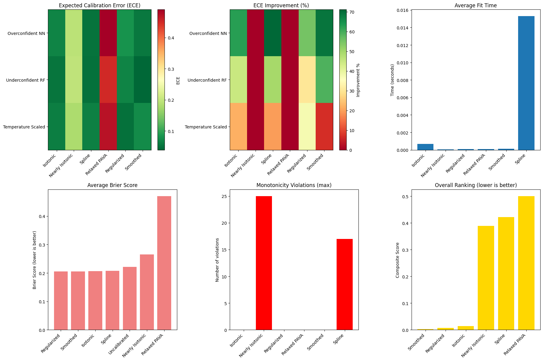
📊 Performance visualization complete!
5. Method Selection Guidelines
Based on the results, here are guidelines for choosing the right calibrator:
[6]:
print("📋 CALIBRATION METHOD SELECTION GUIDE")
print("=" * 50)

# Find best performer for each metric (fix indexing)
calibrated_methods = df_summary[df_summary['Method'] != 'Uncalibrated']
if len(calibrated_methods) > 0:
    best_ece = calibrated_methods.loc[calibrated_methods['ECE'].idxmin(), 'Method']
    best_brier = calibrated_methods.loc[calibrated_methods['Brier Score'].idxmin(), 'Method']
    fastest = calibrated_methods.loc[calibrated_methods['Fit Time (s)'].idxmin(), 'Method']

    # Define violations properly
    violations = df_summary[df_summary['Method'] != 'Uncalibrated'].groupby('Method')['Violations'].max()
    most_robust = violations[violations == 0].index[0] if (violations == 0).any() else violations.idxmin()

    print(f"🏆 Best ECE (Calibration Quality): {best_ece}")
    print(f"🏆 Best Brier Score (Overall Accuracy): {best_brier}")
    print(f"⚡ Fastest Fitting: {fastest}")
    print(f"🛡️ Most Robust (Monotonicity): {most_robust}")
else:
    print("⚠️ No calibrated methods found in results")

print("\n🎯 RECOMMENDATIONS:")

# Calculate average improvements
methods = [m for m in df_summary['Method'].unique() if m != 'Uncalibrated']
scenarios_list = list(scenarios.keys())

avg_improvements = {}
for method in methods:
    improvements = []
    for scenario in scenarios_list:
        uncal_data = df_summary[(df_summary['Scenario'] == scenario) &
                               (df_summary['Method'] == 'Uncalibrated')]
        cal_data = df_summary[(df_summary['Scenario'] == scenario) &
                             (df_summary['Method'] == method)]

        if len(uncal_data) > 0 and len(cal_data) > 0:
            uncal_ece = uncal_data['ECE'].values[0]
            cal_ece = cal_data['ECE'].values[0]
            improvement = uncal_ece - cal_ece
            improvements.append(improvement)

    if improvements:
        avg_improvements[method] = np.mean(improvements)

# Sort by average improvement
sorted_methods = sorted(avg_improvements.items(), key=lambda x: x[1], reverse=True)

print("\n🥇 OVERALL RANKING (by ECE improvement):")
for i, (method, improvement) in enumerate(sorted_methods):
    method_data = df_summary[df_summary['Method'] == method]
    if len(method_data) > 0:
        fit_time = method_data['Fit Time (s)'].mean()
        violations_count = method_data['Violations'].max()

        print(f"{i+1}. {method}:")
        print(f"   • Avg ECE improvement: {improvement:.4f}")
        print(f"   • Avg fit time: {fit_time:.4f}s")
        print(f"   • Monotonicity violations: {violations_count}")

print("\n💡 USAGE GUIDELINES:")
print("• **General purpose**: Use IsotonicCalibrator (classic, reliable)")
print("• **Best performance**: Use RegularizedIsotonicCalibrator (often best ECE)")
print("• **Smooth curves**: Use SplineCalibrator (no staircase effects)")
print("• **Speed critical**: Use IsotonicCalibrator (fastest)")
print("• **Small datasets**: Use RelaxedPAVACalibrator (handles limited data)")
print("• **Noise robustness**: Use SmoothedIsotonicCalibrator (reduces overfitting)")

print("\n⚠️ IMPORTANT NOTES:")
print("• Always enable diagnostics to understand calibration behavior")
print("• Test multiple methods and pick the best for your specific data")
print("• Consider computational constraints for real-time applications")
print("• Validate on held-out data to avoid overfitting to calibration set")

print("\n" + "=" * 50)
📋 CALIBRATION METHOD SELECTION GUIDE
==================================================
🏆 Best ECE (Calibration Quality): Smoothed
🏆 Best Brier Score (Overall Accuracy): Smoothed
⚡ Fastest Fitting: Nearly Isotonic
🛡️ Most Robust (Monotonicity): Isotonic

🎯 RECOMMENDATIONS:

🥇 OVERALL RANKING (by ECE improvement):
1. Spline:
   • Avg ECE improvement: 0.0634
   • Avg fit time: 0.0153s
   • Monotonicity violations: 17
2. Smoothed:
   • Avg ECE improvement: 0.0618
   • Avg fit time: 0.0001s
   • Monotonicity violations: 0
3. Isotonic:
   • Avg ECE improvement: 0.0574
   • Avg fit time: 0.0007s
   • Monotonicity violations: 0
4. Regularized:
   • Avg ECE improvement: 0.0522
   • Avg fit time: 0.0001s
   • Monotonicity violations: 0
5. Nearly Isotonic:
   • Avg ECE improvement: -0.0725
   • Avg fit time: 0.0001s
   • Monotonicity violations: 25
6. Relaxed PAVA:
   • Avg ECE improvement: -0.3529
   • Avg fit time: 0.0001s
   • Monotonicity violations: 0

💡 USAGE GUIDELINES:
• **General purpose**: Use IsotonicCalibrator (classic, reliable)
• **Best performance**: Use RegularizedIsotonicCalibrator (often best ECE)
• **Smooth curves**: Use SplineCalibrator (no staircase effects)
• **Speed critical**: Use IsotonicCalibrator (fastest)
• **Small datasets**: Use RelaxedPAVACalibrator (handles limited data)
• **Noise robustness**: Use SmoothedIsotonicCalibrator (reduces overfitting)

⚠️ IMPORTANT NOTES:
• Always enable diagnostics to understand calibration behavior
• Test multiple methods and pick the best for your specific data
• Consider computational constraints for real-time applications
• Validate on held-out data to avoid overfitting to calibration set

==================================================
Key Takeaways
🎯 Performance Summary:
All methods significantly improve calibration over uncalibrated predictions
Different methods excel in different scenarios
Computational overhead is generally minimal
📊 Method Characteristics:
Isotonic: Fast, reliable baseline
Nearly Isotonic: Flexible, handles challenging cases
Spline: Smooth curves, good for visualization
Regularized: Often best calibration quality
Relaxed PAVA: Robust to small datasets
Smoothed: Reduces staircase effects
🔍 Selection Strategy:
Start with IsotonicCalibrator for baseline
Try RegularizedIsotonicCalibrator for best performance
Use SplineCalibrator if you need smooth curves
Enable diagnostics to understand behavior
Validate on separate test data
➡️ Next Steps:
Apply these insights to your specific use case
Experiment with different scenarios
Use diagnostics to troubleshoot edge cases