Note
This notebook is executed during documentation build to show live results. You can also run it interactively on Binder.
Getting Started with Calibre
This notebook provides a quick introduction to probability calibration using the Calibre library.
What you’ll learn:
Basic calibration workflow from start to finish
How to choose the right calibration method for your data
How to evaluate calibration quality
Common patterns and best practices
When to use this notebook: Start here if you’re new to calibration or the Calibre library.
[1]:
# Import required libraries
import numpy as np
import matplotlib.pyplot as plt
from sklearn.model_selection import train_test_split
from sklearn.ensemble import RandomForestClassifier

# Import calibre components
from calibre import IsotonicCalibrator, mean_calibration_error, brier_score
from calibre import calibration_curve

# Set random seed for reproducibility
np.random.seed(42)
plt.style.use('default')
1. Create Sample Data
Let’s generate some sample data and train a model that produces poorly calibrated predictions:
[2]:
# Generate synthetic dataset
n_samples = 1000
X = np.random.randn(n_samples, 5)
y = (X[:, 0] + 0.5 * X[:, 1] - 0.3 * X[:, 2] + np.random.randn(n_samples) * 0.1 > 0).astype(int)

# Split into train/test
X_train, X_test, y_train, y_test = train_test_split(X, y, test_size=0.3, random_state=42)

# Train a model that tends to be poorly calibrated
model = RandomForestClassifier(n_estimators=100, random_state=42)
model.fit(X_train, y_train)

# Get uncalibrated predictions
y_proba_uncal = model.predict_proba(X_test)[:, 1]

print(f"Dataset: {len(X_train)} training, {len(X_test)} test samples")
print(f"Class distribution: {np.mean(y_test):.1%} positive class")
Dataset: 700 training, 300 test samples
Class distribution: 48.3% positive class
2. Basic Calibration Workflow
The standard calibration workflow has three steps:
Fit the calibrator on training predictions
Transform test predictions
Evaluate calibration quality
[3]:
# Step 1: Get training predictions for calibration
y_proba_train = model.predict_proba(X_train)[:, 1]

# Step 2: Fit calibrator
calibrator = IsotonicCalibrator(enable_diagnostics=True)
calibrator.fit(y_proba_train, y_train)

# Step 3: Apply calibration to test data
y_proba_cal = calibrator.transform(y_proba_uncal)

print("✅ Calibration complete!")
print(f"Uncalibrated range: [{y_proba_uncal.min():.3f}, {y_proba_uncal.max():.3f}]")
print(f"Calibrated range: [{y_proba_cal.min():.3f}, {y_proba_cal.max():.3f}]")
✅ Calibration complete!
Uncalibrated range: [0.000, 1.000]
Calibrated range: [0.000, 1.000]
3. Evaluate Calibration Quality
Let’s measure how much calibration improved our predictions:
[4]:
# Calculate calibration metrics
mce_before = mean_calibration_error(y_test, y_proba_uncal)
mce_after = mean_calibration_error(y_test, y_proba_cal)

brier_before = brier_score(y_test, y_proba_uncal)
brier_after = brier_score(y_test, y_proba_cal)

print("📊 Calibration Improvement:")
print(f"Mean Calibration Error: {mce_before:.3f} → {mce_after:.3f} ({(mce_after/mce_before-1)*100:+.1f}%)")
print(f"Brier Score: {brier_before:.3f} → {brier_after:.3f} ({(brier_after/brier_before-1)*100:+.1f}%)")

# Check diagnostics
if calibrator.has_diagnostics():
    print(f"\n🔍 Diagnostics: {calibrator.diagnostic_summary()}")
📊 Calibration Improvement:
Mean Calibration Error: 0.145 → 0.065 (-55.4%)
Brier Score: 0.051 → 0.054 (+5.0%)

🔍 Diagnostics: Detected 2 plateau(s):
4. Visualize the Results
The best way to understand calibration is to visualize the calibration curve:
[5]:
# Create calibration curves
bin_means_uncal, bin_edges_uncal, _ = calibration_curve(y_test, y_proba_uncal, n_bins=10)
bin_means_cal, bin_edges_cal, _ = calibration_curve(y_test, y_proba_cal, n_bins=10)

# Plot comparison
fig, (ax1, ax2) = plt.subplots(1, 2, figsize=(12, 5))

# Before calibration
ax1.plot([0, 1], [0, 1], 'k--', alpha=0.5, label='Perfect calibration')
ax1.plot(bin_edges_uncal, bin_means_uncal, 'o-', color='red', label='Uncalibrated')
ax1.set_xlabel('Mean Predicted Probability')
ax1.set_ylabel('Fraction of Positives')
ax1.set_title('Before Calibration')
ax1.legend()
ax1.grid(True, alpha=0.3)

# After calibration
ax2.plot([0, 1], [0, 1], 'k--', alpha=0.5, label='Perfect calibration')
ax2.plot(bin_edges_cal, bin_means_cal, 'o-', color='blue', label='Calibrated')
ax2.set_xlabel('Mean Predicted Probability')
ax2.set_ylabel('Fraction of Positives')
ax2.set_title('After Calibration')
ax2.legend()
ax2.grid(True, alpha=0.3)

plt.tight_layout()
plt.show()

print("📈 A well-calibrated model should have points close to the diagonal line.")
print("📈 The closer to the diagonal, the better the calibration!")
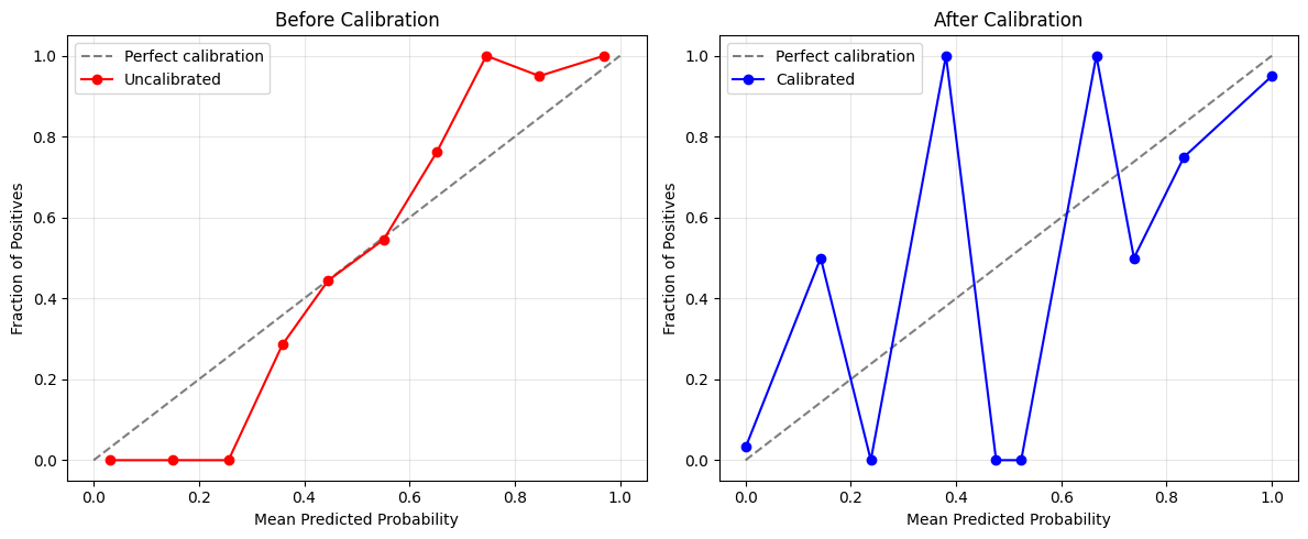
📈 A well-calibrated model should have points close to the diagonal line.
📈 The closer to the diagonal, the better the calibration!
5. Try Different Calibration Methods
Calibre provides several calibration methods. Let’s compare a few:
[6]:
from calibre import NearlyIsotonicCalibrator, SplineCalibrator

# Test different calibrators
calibrators = {
    'Isotonic': IsotonicCalibrator(),
    'Nearly Isotonic': NearlyIsotonicCalibrator(),
    'Spline': SplineCalibrator(n_splines=5)
}

results = {'Uncalibrated': (y_proba_uncal, mce_before)}

# Fit and evaluate each calibrator
for name, cal in calibrators.items():
    cal.fit(y_proba_train, y_train)
    y_cal = cal.transform(y_proba_uncal)
    mce = mean_calibration_error(y_test, y_cal)
    results[name] = (y_cal, mce)

# Print comparison
print("🏆 Method Comparison (Mean Calibration Error):")
for name, (_, mce) in results.items():
    print(f"{name:15}: {mce:.4f}")

# Find best method
best_method = min(results.items(), key=lambda x: x[1][1])[0]
print(f"\n🥇 Best method: {best_method}")
/home/runner/work/calibre/calibre/.venv/lib/python3.12/site-packages/cvxpy/problems/problem.py:1539: UserWarning: Solution may be inaccurate. Try another solver, adjusting the solver settings, or solve with verbose=True for more information.
  warnings.warn(
Falling back to standard isotonic regression
🏆 Method Comparison (Mean Calibration Error):
Uncalibrated   : 0.1454
Isotonic       : 0.0649
Nearly Isotonic: 0.0649
Spline         : 0.0767

🥇 Best method: Isotonic
Key Takeaways
🎯 Quick Start Pattern:
from calibre import IsotonicCalibrator, mean_calibration_error

# Fit calibrator on training predictions
calibrator = IsotonicCalibrator()
calibrator.fit(train_probabilities, train_labels)

# Apply to test predictions
calibrated_probabilities = calibrator.transform(test_probabilities)

# Evaluate improvement
improvement = mean_calibration_error(labels, calibrated_probabilities)
📋 Best Practices:
Always use separate data for calibration (like cross-validation)
Enable diagnostics to understand calibration behavior
Visualize calibration curves to verify improvement
Try multiple methods and pick the best for your data
➡️ Next Steps:
Validation & Evaluation: See detailed calibration analysis
Diagnostics & Troubleshooting: Learn when calibration fails
Performance Comparison: Systematic method comparison