Choosing a binary threshold on held-out data

A classifier’s default 0.5 cutoff is rarely the one that maximizes F1 when positives are rare. optimize_thresholds finds the F1-maximizing cutoff exactly, but only data it did not see can say how well that cutoff does: tuning on the test set and scoring on it reports that set’s own maximum.

Three splits: fit the model, choose the cutoff, measure

import matplotlib.pyplot as plt
import numpy as np
from sklearn.datasets import make_classification
from sklearn.linear_model import LogisticRegression
from sklearn.metrics import f1_score
from sklearn.model_selection import train_test_split

from optimal_cutoffs import optimize_thresholds

X, y = make_classification(
    n_samples=6000, weights=[0.9], class_sep=0.8, flip_y=0.02, random_state=0
)
X_train, X_rest, y_train, y_rest = train_test_split(
    X, y, test_size=0.5, stratify=y, random_state=0
)
X_val, X_test, y_val, y_test = train_test_split(
    X_rest, y_rest, test_size=0.5, stratify=y_rest, random_state=0
)
model = LogisticRegression().fit(X_train, y_train)
p_val = model.predict_proba(X_val)[:, 1]
p_test = model.predict_proba(X_test)[:, 1]

tuned = optimize_thresholds(y_val, p_val, metric="f1")
peeked = optimize_thresholds(y_test, p_test, metric="f1")

print(f"positives: {y_test.mean():.1%} of the test set")
print(f"{'cutoff':<28} {'value':>6} {'test F1':>8}")
for label, cutoff in [
    ("default", 0.5),
    ("tuned on validation", tuned.threshold),
    ("tuned on test (optimistic)", peeked.threshold),
]:
    print(f"{label:<28} {cutoff:6.3f} {f1_score(y_test, p_test > cutoff):8.3f}")

positives: 10.7% of the test set
cutoff                        value  test F1
default                       0.500    0.424
tuned on validation           0.239    0.529
tuned on test (optimistic)    0.206    0.549

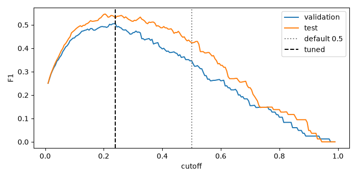
F1 against the cutoff

The validation and test curves peak in different places; the gap between the optimistic row above and the validation-tuned row is how much tuning on the test set would overstate F1.

grid = np.linspace(0.01, 0.99, 197)
fig, ax = plt.subplots(figsize=(7, 3.5))
ax.plot(grid, [f1_score(y_val, p_val > t) for t in grid], label="validation")
ax.plot(grid, [f1_score(y_test, p_test > t) for t in grid], label="test")
ax.axvline(0.5, color="gray", linestyle=":", label="default 0.5")
ax.axvline(tuned.threshold, color="black", linestyle="--", label="tuned")
ax.set_xlabel("cutoff")
ax.set_ylabel("F1")
ax.legend()
fig.tight_layout()
plt.show()

Costs instead of F1

When a missed positive costs ten times a false alarm and the probabilities are calibrated, the cost-minimizing cutoff is known in closed form: 1 / (1 + 10). mode="bayes" returns it without looking at labels.

bayes = optimize_thresholds(
    None, p_test, mode="bayes", utility={"tp": 0, "tn": 0, "fp": -1, "fn": -10}
)


def mean_cost(cutoff):
    pred = p_test > cutoff
    return ((pred & (y_test == 0)).sum() + 10 * (~pred & (y_test == 1)).sum()) / len(
        y_test
    )


print(f"Bayes cutoff {bayes.threshold:.4f} (1/11 = {1 / 11:.4f})")
print(f"mean cost per case: {mean_cost(0.5):.3f} at 0.5, ", end="")
print(f"{mean_cost(bayes.threshold):.3f} at the Bayes cutoff")

Bayes cutoff 0.0909 (1/11 = 0.0909)
mean cost per case: 0.751 at 0.5, 0.328 at the Bayes cutoff