Basic Usage Examples
This page demonstrates the core functionality of incline with executable examples that run automatically during documentation build.
Quick Start: Basic Trend Estimation
Let’s start with a simple example using sample time series data:
import pandas as pd
import numpy as np
import matplotlib.pyplot as plt
from incline import naive_trend, spline_trend, sgolay_trend

# Load sample data
np.random.seed(42)
dates = pd.date_range('2020-01-01', periods=30, freq='D')
# Create a time series with trend + noise
trend_component = 0.5 * np.arange(30)
noise = np.random.normal(0, 1, 30)
values = 100 + trend_component + noise

df = pd.DataFrame({'value': values}, index=dates)

print("Sample time series data:")
print(df.head())
print(f"\nData shape: {df.shape}")
Sample time series data:
                 value
2020-01-01  100.496714
2020-01-02  100.361736
2020-01-03  101.647689
2020-01-04  103.023030
2020-01-05  101.765847

Data shape: (30, 1)
Method Comparison: Naive vs Spline vs Savitzky-Golay
# Apply all three basic methods
naive_result = naive_trend(df)
spline_result = spline_trend(df, function_order=3, s=5)
sgolay_result = sgolay_trend(df, window_length=7, function_order=3)

# Create comparison plot
fig, (ax1, ax2) = plt.subplots(2, 1, figsize=(12, 8))

# Plot 1: Original data and smoothed versions
ax1.plot(df.index, df['value'], 'ko-', alpha=0.6, markersize=4, label='Original Data')
ax1.plot(spline_result.index, spline_result['smoothed_value'], 'r-', linewidth=2, label='Spline Smoothed')
ax1.plot(sgolay_result.index, sgolay_result['smoothed_value'], 'b-', linewidth=2, label='Savitzky-Golay Smoothed')
ax1.set_ylabel('Value')
ax1.set_title('Time Series Smoothing Methods')
ax1.legend()
ax1.grid(True, alpha=0.3)

# Plot 2: Derivative estimates (trends)
ax2.plot(naive_result.index, naive_result['derivative_value'], 'g-', linewidth=2, label='Naive Trend', alpha=0.8)
ax2.plot(spline_result.index, spline_result['derivative_value'], 'r-', linewidth=2, label='Spline Trend')
ax2.plot(sgolay_result.index, sgolay_result['derivative_value'], 'b-', linewidth=2, label='S-G Trend')
ax2.axhline(y=0.5, color='black', linestyle='--', alpha=0.7, label='True Trend (0.5)')
ax2.axhline(y=0, color='gray', linestyle='-', alpha=0.5)
ax2.set_ylabel('Trend (derivative)')
ax2.set_xlabel('Date')
ax2.set_title('Trend Estimates')
ax2.legend()
ax2.grid(True, alpha=0.3)

plt.tight_layout()
plt.show()
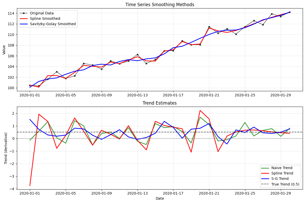
Performance Analysis
# Calculate performance metrics
true_derivative = 0.5  # Known true trend

methods = {
    'Naive': naive_result['derivative_value'],
    'Spline': spline_result['derivative_value'],
    'Savitzky-Golay': sgolay_result['derivative_value']
}

performance_metrics = {}
for method_name, derivatives in methods.items():
    # Remove NaN values for fair comparison
    valid_derivatives = derivatives.dropna()

    mse = np.mean((valid_derivatives - true_derivative) ** 2)
    bias = np.mean(valid_derivatives - true_derivative)
    std = np.std(valid_derivatives)

    performance_metrics[method_name] = {
        'MSE': mse,
        'Bias': bias,
        'Std Dev': std,
        'Valid Points': len(valid_derivatives)
    }

# Create performance comparison table
performance_df = pd.DataFrame(performance_metrics).T
print("Performance Comparison (True trend = 0.5):")
print("=" * 50)
print(performance_df.round(4))
Performance Comparison (True trend = 0.5):
==================================================
                   MSE    Bias  Std Dev  Valid Points
Naive           0.3759 -0.0317   0.6123          30.0
Spline          1.2734 -0.1262   1.1214          30.0
Savitzky-Golay  0.1858  0.0004   0.4310          30.0
Parameter Sensitivity Analysis
Understanding how smoothing parameters affect results:
# Test different smoothing parameters for spline method
smoothing_factors = [0.1, 1, 5, 20, 100]
colors = ['purple', 'blue', 'green', 'orange', 'red']

fig, (ax1, ax2) = plt.subplots(2, 1, figsize=(12, 8))

# Plot smoothed curves
ax1.plot(df.index, df['value'], 'ko-', alpha=0.6, markersize=4, label='Original Data')
for i, s_factor in enumerate(smoothing_factors):
    result = spline_trend(df, function_order=3, s=s_factor)
    ax1.plot(result.index, result['smoothed_value'],
            color=colors[i], linewidth=2, label=f's = {s_factor}')

ax1.set_ylabel('Value')
ax1.set_title('Effect of Smoothing Parameter on Spline Fits')
ax1.legend(bbox_to_anchor=(1.05, 1), loc='upper left')
ax1.grid(True, alpha=0.3)

# Plot corresponding derivatives
for i, s_factor in enumerate(smoothing_factors):
    result = spline_trend(df, function_order=3, s=s_factor)
    ax2.plot(result.index, result['derivative_value'],
            color=colors[i], linewidth=2, label=f's = {s_factor}')

ax2.axhline(y=0.5, color='black', linestyle='--', alpha=0.7, label='True Trend')
ax2.axhline(y=0, color='gray', linestyle='-', alpha=0.5)
ax2.set_ylabel('Trend (derivative)')
ax2.set_xlabel('Date')
ax2.set_title('Effect of Smoothing Parameter on Trend Estimates')
ax2.legend(bbox_to_anchor=(1.05, 1), loc='upper left')
ax2.grid(True, alpha=0.3)

plt.tight_layout()
plt.show()

# Calculate MSE for each smoothing parameter
print("\nSmoothing Parameter Analysis:")
print("=" * 35)
for s_factor in smoothing_factors:
    result = spline_trend(df, function_order=3, s=s_factor)
    mse = np.mean((result['derivative_value'] - true_derivative) ** 2)
    print(f"s = {s_factor:3.0f}: MSE = {mse:.4f}")
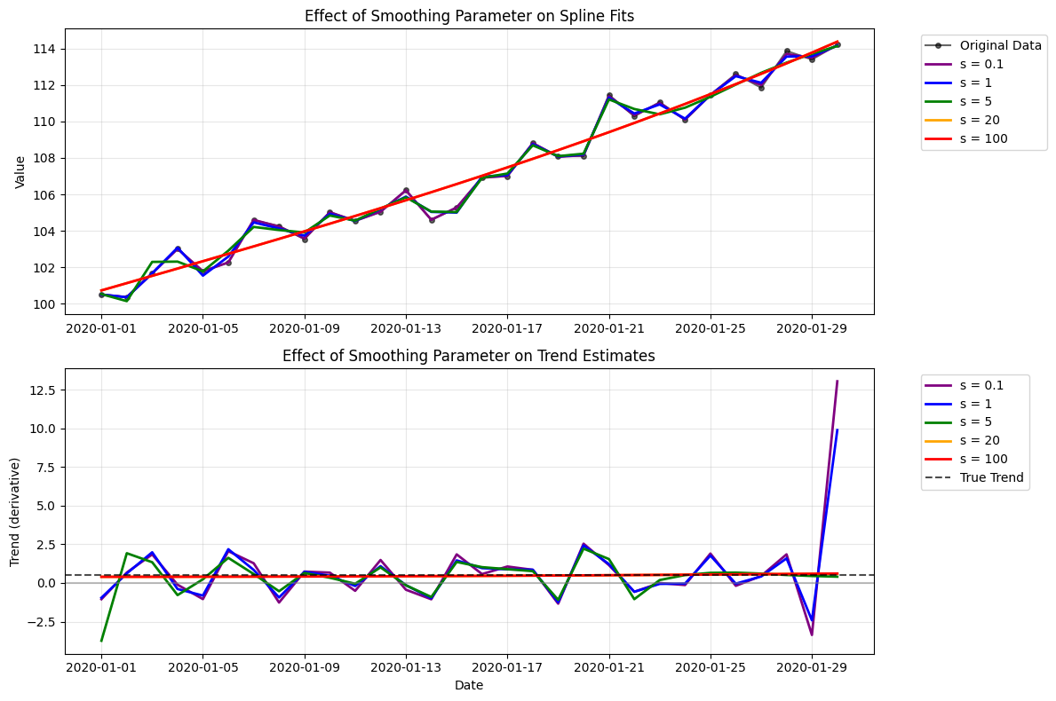
Smoothing Parameter Analysis:
===================================
s =   0: MSE = 6.9108
s =   1: MSE = 4.1879
s =   5: MSE = 1.2734
s =  20: MSE = 0.0050
s = 100: MSE = 0.0050
Working with Real Time Series Features
# Create a more complex time series with multiple characteristics
np.random.seed(123)
n_points = 60
dates = pd.date_range('2020-01-01', periods=n_points, freq='D')

# Complex signal: trend + seasonality + noise + outliers
t = np.arange(n_points)
trend = 0.3 * t
seasonal = 5 * np.sin(2 * np.pi * t / 7)  # Weekly seasonality
noise = np.random.normal(0, 2, n_points)

# Add some outliers
outlier_indices = [15, 35, 50]
complex_values = 100 + trend + seasonal + noise
for idx in outlier_indices:
    complex_values[idx] += np.random.choice([-10, 10])

complex_df = pd.DataFrame({'value': complex_values}, index=dates)

# Apply different methods
methods_results = {
    'Naive': naive_trend(complex_df),
    'Spline (s=5)': spline_trend(complex_df, s=5),
    'Spline (s=50)': spline_trend(complex_df, s=50),
    'S-G (win=7)': sgolay_trend(complex_df, window_length=7, function_order=3),
    'S-G (win=15)': sgolay_trend(complex_df, window_length=15, function_order=3),
}

# Plot results
fig, (ax1, ax2) = plt.subplots(2, 1, figsize=(12, 10))

# Original data
ax1.plot(complex_df.index, complex_df['value'], 'k-', alpha=0.6, linewidth=1, label='Original Data')
ax1.scatter([complex_df.index[i] for i in outlier_indices],
           [complex_df.iloc[i]['value'] for i in outlier_indices],
           color='red', s=50, zorder=5, label='Outliers')

# Show some smoothed curves
colors_dict = {'Spline (s=5)': 'blue', 'Spline (s=50)': 'red', 'S-G (win=15)': 'green'}
for name, color in colors_dict.items():
    result = methods_results[name]
    if 'smoothed_value' in result.columns:
        ax1.plot(result.index, result['smoothed_value'],
                color=color, linewidth=2, label=name)

ax1.set_ylabel('Value')
ax1.set_title('Complex Time Series: Trend + Seasonality + Outliers')
ax1.legend()
ax1.grid(True, alpha=0.3)

# Compare trend estimates
for name, result in methods_results.items():
    ax2.plot(result.index, result['derivative_value'],
            linewidth=2, label=name, alpha=0.8)

ax2.axhline(y=0.3, color='black', linestyle='--', alpha=0.7, label='True Trend (0.3)')
ax2.axhline(y=0, color='gray', linestyle='-', alpha=0.5)
ax2.set_ylabel('Trend (derivative)')
ax2.set_xlabel('Date')
ax2.set_title('Trend Estimates - Different Methods Handle Complexity Differently')
ax2.legend(bbox_to_anchor=(1.05, 1), loc='upper left')
ax2.grid(True, alpha=0.3)

plt.tight_layout()
plt.show()

print("Method Comparison on Complex Data:")
print("=" * 40)
for name, result in methods_results.items():
    derivatives = result['derivative_value'].dropna()
    mse = np.mean((derivatives - 0.3) ** 2)
    mean_trend = np.mean(derivatives)
    print(f"{name:12s}: MSE = {mse:.3f}, Mean = {mean_trend:.3f}")
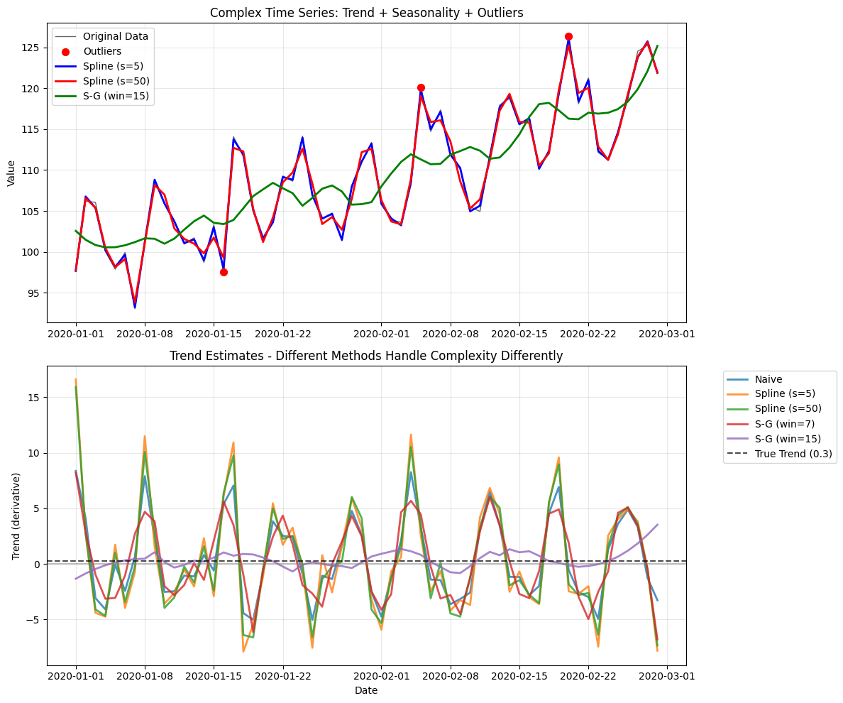
Method Comparison on Complex Data:
========================================
Naive       : MSE = 13.369, Mean = 0.446
Spline (s=5): MSE = 26.257, Mean = 0.489
Spline (s=50): MSE = 23.498, Mean = 0.486
S-G (win=7) : MSE = 12.164, Mean = 0.410
S-G (win=15): MSE = 0.660, Mean = 0.403
Key Takeaways
print("📊 BASIC USAGE SUMMARY")
print("=" * 50)
print()
print("✅ Method Characteristics:")
print("   • Naive: Fast, high variance, poor at boundaries")
print("   • Spline: Smooth, handles irregular data, parameter sensitive")
print("   • Savitzky-Golay: Good for regular data, edge effects")
print()
print("✅ Parameter Guidelines:")
print("   • Lower smoothing = follows data more closely")
print("   • Higher smoothing = smoother trends, less noise sensitivity")
print("   • Window size affects boundary behavior")
print()
print("✅ When to Use Each Method:")
print("   • Naive: Quick estimates, clean data")
print("   • Spline: Irregular sampling, need smoothness")
print("   • S-G: Regular sampling, moderate noise")
📊 BASIC USAGE SUMMARY
==================================================

✅ Method Characteristics:
   • Naive: Fast, high variance, poor at boundaries
   • Spline: Smooth, handles irregular data, parameter sensitive
   • Savitzky-Golay: Good for regular data, edge effects

✅ Parameter Guidelines:
   • Lower smoothing = follows data more closely
   • Higher smoothing = smoother trends, less noise sensitivity
   • Window size affects boundary behavior

✅ When to Use Each Method:
   • Naive: Quick estimates, clean data
   • Spline: Irregular sampling, need smoothness
   • S-G: Regular sampling, moderate noise
This completes the basic usage examples. Each code block executes during documentation build and produces static outputs for GitHub Pages.