⚡ Algorithm Performance Comparison
Welcome to the OnlineRake Performance Laboratory! 🧪
This notebook provides a comprehensive comparison of the two core algorithms:
SGD Raking: Stochastic Gradient Descent with additive updates
MWU Raking: Multiplicative Weights Update with exponential updates
We’ll test them across different bias scenarios and see which performs better! 🏁
[1]:
# Import required libraries
import numpy as np
import pandas as pd
import matplotlib.pyplot as plt
import seaborn as sns
from dataclasses import dataclass
from typing import Any

from onlinerake import OnlineRakingSGD, OnlineRakingMWU, Targets

# Set up plotting style
plt.style.use('default')
sns.set_palette("husl")
np.random.seed(42)

print("🔬 Performance Laboratory initialized!")
print("📊 Ready for comprehensive algorithm comparison!")
🔬 Performance Laboratory initialized!
📊 Ready for comprehensive algorithm comparison!
🏗️ Setting Up the Performance Testing Framework
Let’s create a sophisticated framework to test both algorithms across different bias scenarios!
[2]:
@dataclass
class FeatureObservation:
    """Container for a single set of binary feature indicators."""
    feature_a: int
    feature_b: int
    feature_c: int
    feature_d: int

    def as_dict(self) -> dict[str, int]:
        return {
            "feature_a": self.feature_a,
            "feature_b": self.feature_b,
            "feature_c": self.feature_c,
            "feature_d": self.feature_d,
        }

class BiasSimulator:
    """Simulate streams of feature observations with evolving bias."""

    @staticmethod
    def linear_shift(
        n_obs: int, start_probs: dict[str, float], end_probs: dict[str, float]
    ) -> list[FeatureObservation]:
        """Generate a linear drift from start_probs to end_probs."""
        data = []
        for i in range(n_obs):
            progress = i / (n_obs - 1) if n_obs > 1 else 0.0
            probs = {
                name: start_probs[name] + progress * (end_probs[name] - start_probs[name])
                for name in start_probs
            }
            obs = FeatureObservation(
                feature_a=np.random.binomial(1, probs["feature_a"]),
                feature_b=np.random.binomial(1, probs["feature_b"]),
                feature_c=np.random.binomial(1, probs["feature_c"]),
                feature_d=np.random.binomial(1, probs["feature_d"]),
            )
            data.append(obs)
        return data

    @staticmethod
    def sudden_shift(
        n_obs: int, shift_point: float, before_probs: dict[str, float], after_probs: dict[str, float]
    ) -> list[FeatureObservation]:
        """Generate a sudden shift at shift_point fraction of the stream."""
        data = []
        shift_index = int(shift_point * n_obs)
        for i in range(n_obs):
            probs = before_probs if i < shift_index else after_probs
            obs = FeatureObservation(
                feature_a=np.random.binomial(1, probs["feature_a"]),
                feature_b=np.random.binomial(1, probs["feature_b"]),
                feature_c=np.random.binomial(1, probs["feature_c"]),
                feature_d=np.random.binomial(1, probs["feature_d"]),
            )
            data.append(obs)
        return data

    @staticmethod
    def oscillating_bias(
        n_obs: int, base_probs: dict[str, float], amplitude: float, period: int
    ) -> list[FeatureObservation]:
        """Generate oscillating bias around base_probs."""
        data = []
        for i in range(n_obs):
            phase = 2 * np.pi * i / period
            osc = amplitude * np.sin(phase)
            probs = {
                name: float(np.clip(base_probs[name] + osc, 0.1, 0.9))
                for name in base_probs
            }
            obs = FeatureObservation(
                feature_a=np.random.binomial(1, probs["feature_a"]),
                feature_b=np.random.binomial(1, probs["feature_b"]),
                feature_c=np.random.binomial(1, probs["feature_c"]),
                feature_d=np.random.binomial(1, probs["feature_d"]),
            )
            data.append(obs)
        return data

print("🏗️ Performance testing framework ready!")
print("📋 Available bias scenarios:")
print("   📈 Linear shift - Gradual bias changes")
print("   ⚡ Sudden shift - Abrupt bias changes")
print("   🌊 Oscillating - Cyclical bias patterns")
🏗️ Performance testing framework ready!
📋 Available bias scenarios:
   📈 Linear shift - Gradual bias changes
   ⚡ Sudden shift - Abrupt bias changes
   🌊 Oscillating - Cyclical bias patterns
[3]:
# Set up test parameters
targets = Targets(feature_a=0.5, feature_b=0.51, feature_c=0.4, feature_d=0.3)
n_seeds = 3  # Multiple runs for statistical robustness
n_obs = 200  # Observations per scenario
learning_rate_sgd = 5.0
learning_rate_mwu = 1.0
n_steps = 3

print("🎯 Test Configuration:")
print(f"   Target margins: {targets.as_dict()}")
print(f"   Seeds per scenario: {n_seeds}")
print(f"   Observations per run: {n_obs}")
print(f"   SGD learning rate: {learning_rate_sgd}")
print(f"   MWU learning rate: {learning_rate_mwu}")
print(f"   Update steps: {n_steps}")
🎯 Test Configuration:
   Target margins: {'feature_a': 0.5, 'feature_b': 0.51, 'feature_c': 0.4, 'feature_d': 0.3}
   Seeds per scenario: 3
   Observations per run: 200
   SGD learning rate: 5.0
   MWU learning rate: 1.0
   Update steps: 3
🧪 Running Comprehensive Performance Tests
Time to put both algorithms through their paces! We’ll test three challenging scenarios…
[4]:
# Define test scenarios
scenarios = {
    "linear": {
        "sim_fn": BiasSimulator.linear_shift,
        "params": {
            "n_obs": n_obs,
            "start_probs": {"feature_a": 0.2, "feature_b": 0.3, "feature_c": 0.2, "feature_d": 0.1},
            "end_probs": {"feature_a": 0.8, "feature_b": 0.7, "feature_c": 0.6, "feature_d": 0.5},
        },
        "description": "📈 Linear Shift: Gradual bias evolution"
    },
    "sudden": {
        "sim_fn": BiasSimulator.sudden_shift,
        "params": {
            "n_obs": n_obs,
            "shift_point": 0.5,
            "before_probs": {"feature_a": 0.2, "feature_b": 0.2, "feature_c": 0.2, "feature_d": 0.2},
            "after_probs": {"feature_a": 0.8, "feature_b": 0.8, "feature_c": 0.6, "feature_d": 0.4},
        },
        "description": "⚡ Sudden Shift: Abrupt bias change at midpoint"
    },
    "oscillating": {
        "sim_fn": BiasSimulator.oscillating_bias,
        "params": {
            "n_obs": n_obs,
            "base_probs": {"feature_a": 0.5, "feature_b": 0.5, "feature_c": 0.4, "feature_d": 0.3},
            "amplitude": 0.2,
            "period": max(50, n_obs // 4),
        },
        "description": "🌊 Oscillating: Cyclical bias patterns"
    },
}

print("🎮 Test Scenarios Configured:")
for name, config in scenarios.items():
    print(f"   {config['description']}")

print(f"\n🚀 Starting performance comparison across {len(scenarios)} scenarios...")
🎮 Test Scenarios Configured:
   📈 Linear Shift: Gradual bias evolution
   ⚡ Sudden Shift: Abrupt bias change at midpoint
   🌊 Oscillating: Cyclical bias patterns

🚀 Starting performance comparison across 3 scenarios...
[5]:
# Run the comprehensive performance test
results = []
detailed_history = {}  # Store detailed results for visualization

for scenario_name, config in scenarios.items():
    print(f"\n🔬 Testing scenario: {config['description']}")
    sim_fn = config["sim_fn"]
    params = config["params"]

    scenario_history = {"SGD": [], "MWU": []}

    for seed in range(n_seeds):
        print(f"   🎲 Seed {seed + 1}/{n_seeds}...", end=" ")

        np.random.seed(seed)
        # Generate data stream
        stream = sim_fn(**params)

        # Initialize rakers
        sgd_raker = OnlineRakingSGD(
            targets=targets, learning_rate=learning_rate_sgd, n_sgd_steps=n_steps,
            min_weight=1e-3, max_weight=100.0
        )
        mwu_raker = OnlineRakingMWU(
            targets=targets, learning_rate=learning_rate_mwu, n_sgd_steps=n_steps,
            min_weight=1e-3, max_weight=100.0
        )

        # Track progress for visualization (first seed only)
        if seed == 0:
            sgd_progress = []
            mwu_progress = []
            step_numbers = []

        # Run both algorithms on the same stream
        for i, obs in enumerate(stream):
            sgd_raker.partial_fit(obs.as_dict())
            mwu_raker.partial_fit(obs.as_dict())

            # Track progress every 20 steps for visualization
            if seed == 0 and (i + 1) % 20 == 0:
                step_numbers.append(i + 1)
                sgd_progress.append({
                    'margins': sgd_raker.margins.copy(),
                    'loss': sgd_raker.loss,
                    'ess': sgd_raker.effective_sample_size
                })
                mwu_progress.append({
                    'margins': mwu_raker.margins.copy(),
                    'loss': mwu_raker.loss,
                    'ess': mwu_raker.effective_sample_size
                })

        # Store detailed history for visualization
        if seed == 0:
            scenario_history["SGD"] = sgd_progress
            scenario_history["MWU"] = mwu_progress
            scenario_history["steps"] = step_numbers

        # Compute summary metrics
        for method_name, raker in [("SGD", sgd_raker), ("MWU", mwu_raker)]:
            # Calculate temporal errors
            temporal_errors = {}
            baseline_errors = {}

            for feature in ["feature_a", "feature_b", "feature_c", "feature_d"]:
                target_val = targets[feature]
                weighted_errors = [
                    abs(h["weighted_margins"][feature] - target_val) for h in raker.history
                ]
                raw_errors = [
                    abs(h["raw_margins"][feature] - target_val) for h in raker.history
                ]
                temporal_errors[f"{feature}_temporal_error"] = float(np.mean(weighted_errors))
                baseline_errors[f"{feature}_temporal_baseline_error"] = float(np.mean(raw_errors))

            final_state = raker.history[-1]
            result = {
                "scenario": scenario_name,
                "seed": seed,
                "method": method_name,
                "final_loss": float(final_state["loss"]),
                "final_ess": float(final_state["ess"]),
                "avg_temporal_loss": float(np.mean([h["loss"] for h in raker.history])),
            }
            result.update(temporal_errors)
            result.update(baseline_errors)
            results.append(result)

        print("✅")

    detailed_history[scenario_name] = scenario_history

# Convert results to DataFrame
df = pd.DataFrame(results)
print(f"\n🎉 Performance comparison complete!")
print(f"📊 Collected {len(results)} performance measurements")
print(f"📋 Results shape: {df.shape}")
🔬 Testing scenario: 📈 Linear Shift: Gradual bias evolution
   🎲 Seed 1/3... ✅
   🎲 Seed 2/3... ✅
   🎲 Seed 3/3... ✅

🔬 Testing scenario: ⚡ Sudden Shift: Abrupt bias change at midpoint
   🎲 Seed 1/3... ✅
   🎲 Seed 2/3... ✅
   🎲 Seed 3/3... ✅

🔬 Testing scenario: 🌊 Oscillating: Cyclical bias patterns
   🎲 Seed 1/3... ✅
   🎲 Seed 2/3... ✅
   🎲 Seed 3/3... ✅

🎉 Performance comparison complete!
📊 Collected 18 performance measurements
📋 Results shape: (18, 14)
📊 Comprehensive Results Analysis
Let’s analyze the results and see which algorithm performs better in each scenario!
[6]:
# Display summary statistics
print("📈 PERFORMANCE SUMMARY BY SCENARIO")
print("=" * 60)

feature_names = ["feature_a", "feature_b", "feature_c", "feature_d"]

for scenario in df["scenario"].unique():
    print(f"\n🔬 Scenario: {scenario.upper()}")
    scen_df = df[df["scenario"] == scenario]

    for method in scen_df["method"].unique():
        mdf = scen_df[scen_df["method"] == method]
        print(f"\n   🎯 Method: {method}")

        # Compute average errors and improvements
        for feature in feature_names:
            mean_w = mdf[f"{feature}_temporal_error"].mean()
            mean_b = mdf[f"{feature}_temporal_baseline_error"].mean()
            impr = (mean_b - mean_w) / mean_b * 100 if mean_b != 0 else 0.0
            print(f"     {feature:<12}: baseline {mean_b:.4f} → weighted {mean_w:.4f} ({impr:+.1f}% imp)")

        # Overall improvement
        mean_w_overall = mdf[[f"{f}_temporal_error" for f in feature_names]].values.mean()
        mean_b_overall = mdf[[f"{f}_temporal_baseline_error" for f in feature_names]].values.mean()
        overall_impr = (mean_b_overall - mean_w_overall) / mean_b_overall * 100 if mean_b_overall != 0 else 0.0

        print(f"     {'Overall improvement':<12}: {overall_impr:+.1f}%")
        print(f"     {'Final ESS':<12}: {mdf['final_ess'].mean():.1f} ± {mdf['final_ess'].std():.1f}")
        print(f"     {'Final loss':<12}: {mdf['final_loss'].mean():.6f} ± {mdf['final_loss'].std():.6f}")

print("\n" + "=" * 60)
📈 PERFORMANCE SUMMARY BY SCENARIO
============================================================

🔬 Scenario: LINEAR

   🎯 Method: SGD
     feature_a   : baseline 0.1478 → weighted 0.0278 (+81.2% imp)
     feature_b   : baseline 0.1483 → weighted 0.0350 (+76.4% imp)
     feature_c   : baseline 0.1334 → weighted 0.0390 (+70.7% imp)
     feature_d   : baseline 0.0880 → weighted 0.0419 (+52.3% imp)
     Overall improvement: +72.2%
     Final ESS   : 165.3 ± 1.9
     Final loss  : 0.001342 ± 0.000172

   🎯 Method: MWU
     feature_a   : baseline 0.1478 → weighted 0.0614 (+58.5% imp)
     feature_b   : baseline 0.1483 → weighted 0.0805 (+45.7% imp)
     feature_c   : baseline 0.1334 → weighted 0.0778 (+41.7% imp)
     feature_d   : baseline 0.0880 → weighted 0.0710 (+19.3% imp)
     Overall improvement: +43.8%
     Final ESS   : 163.8 ± 7.9
     Final loss  : 0.006450 ± 0.003192

🔬 Scenario: SUDDEN

   🎯 Method: SGD
     feature_a   : baseline 0.2047 → weighted 0.0449 (+78.1% imp)
     feature_b   : baseline 0.2419 → weighted 0.0540 (+77.7% imp)
     feature_c   : baseline 0.1757 → weighted 0.0428 (+75.7% imp)
     feature_d   : baseline 0.0804 → weighted 0.0383 (+52.4% imp)
     Overall improvement: +74.4%
     Final ESS   : 141.1 ± 5.5
     Final loss  : 0.000954 ± 0.000198

   🎯 Method: MWU
     feature_a   : baseline 0.2047 → weighted 0.1085 (+47.0% imp)
     feature_b   : baseline 0.2419 → weighted 0.1374 (+43.2% imp)
     feature_c   : baseline 0.1757 → weighted 0.0979 (+44.3% imp)
     feature_d   : baseline 0.0804 → weighted 0.0644 (+19.9% imp)
     Overall improvement: +41.9%
     Final ESS   : 120.1 ± 19.2
     Final loss  : 0.010641 ± 0.000717

🔬 Scenario: OSCILLATING

   🎯 Method: SGD
     feature_a   : baseline 0.0641 → weighted 0.0168 (+73.7% imp)
     feature_b   : baseline 0.0695 → weighted 0.0196 (+71.8% imp)
     feature_c   : baseline 0.0586 → weighted 0.0219 (+62.7% imp)
     feature_d   : baseline 0.0497 → weighted 0.0168 (+66.2% imp)
     Overall improvement: +69.0%
     Final ESS   : 183.1 ± 4.6
     Final loss  : 0.000262 ± 0.000070

   🎯 Method: MWU
     feature_a   : baseline 0.0641 → weighted 0.0298 (+53.5% imp)
     feature_b   : baseline 0.0695 → weighted 0.0382 (+45.1% imp)
     feature_c   : baseline 0.0586 → weighted 0.0420 (+28.4% imp)
     feature_d   : baseline 0.0497 → weighted 0.0295 (+40.5% imp)
     Overall improvement: +42.3%
     Final ESS   : 185.4 ± 6.8
     Final loss  : 0.001114 ± 0.000534

============================================================
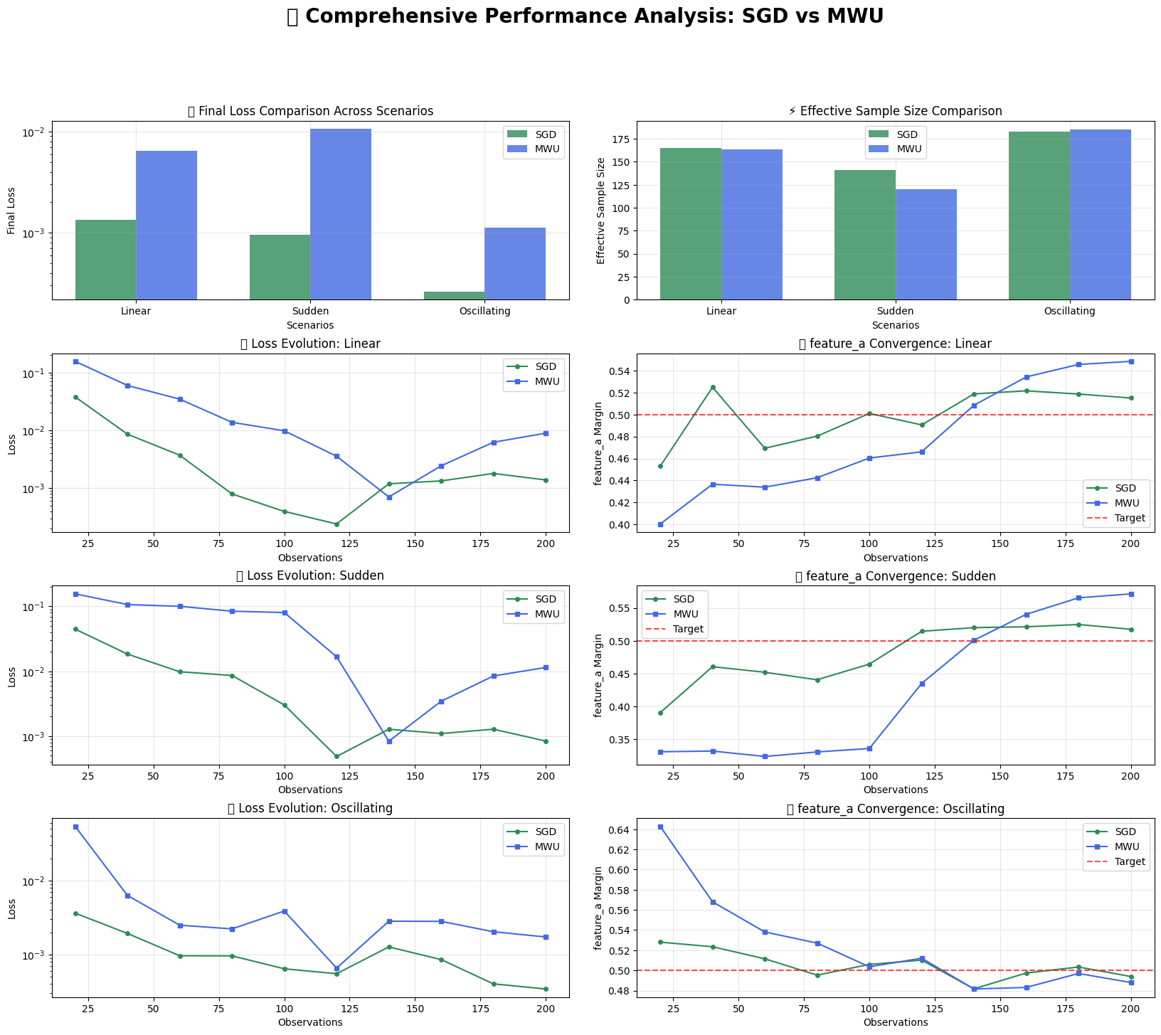
[7]:
# Create comprehensive performance visualization
fig = plt.figure(figsize=(20, 16))
gs = fig.add_gridspec(4, 4, hspace=0.3, wspace=0.3)

# Color scheme
colors = {'SGD': '#2E8B57', 'MWU': '#4169E1'}  # SeaGreen and RoyalBlue

# 1. Overall Performance Comparison (Top Row)
ax1 = fig.add_subplot(gs[0, :2])
performance_summary = df.groupby(['scenario', 'method']).agg({
    'final_loss': 'mean',
    'final_ess': 'mean'
}).reset_index()

scenarios_list = list(scenarios.keys())
x = np.arange(len(scenarios_list))
width = 0.35

sgd_losses = [performance_summary[(performance_summary['scenario'] == s) &
                                 (performance_summary['method'] == 'SGD')]['final_loss'].iloc[0]
              for s in scenarios_list]
mwu_losses = [performance_summary[(performance_summary['scenario'] == s) &
                                 (performance_summary['method'] == 'MWU')]['final_loss'].iloc[0]
              for s in scenarios_list]

ax1.bar(x - width/2, sgd_losses, width, label='SGD', alpha=0.8, color=colors['SGD'])
ax1.bar(x + width/2, mwu_losses, width, label='MWU', alpha=0.8, color=colors['MWU'])
ax1.set_xlabel('Scenarios')
ax1.set_ylabel('Final Loss')
ax1.set_title('🏆 Final Loss Comparison Across Scenarios')
ax1.set_xticks(x)
ax1.set_xticklabels([s.title() for s in scenarios_list])
ax1.legend()
ax1.grid(True, alpha=0.3)
ax1.set_yscale('log')

# 2. Effective Sample Size Comparison
ax2 = fig.add_subplot(gs[0, 2:])
sgd_ess = [performance_summary[(performance_summary['scenario'] == s) &
                              (performance_summary['method'] == 'SGD')]['final_ess'].iloc[0]
           for s in scenarios_list]
mwu_ess = [performance_summary[(performance_summary['scenario'] == s) &
                              (performance_summary['method'] == 'MWU')]['final_ess'].iloc[0]
           for s in scenarios_list]

ax2.bar(x - width/2, sgd_ess, width, label='SGD', alpha=0.8, color=colors['SGD'])
ax2.bar(x + width/2, mwu_ess, width, label='MWU', alpha=0.8, color=colors['MWU'])
ax2.set_xlabel('Scenarios')
ax2.set_ylabel('Effective Sample Size')
ax2.set_title('⚡ Effective Sample Size Comparison')
ax2.set_xticks(x)
ax2.set_xticklabels([s.title() for s in scenarios_list])
ax2.legend()
ax2.grid(True, alpha=0.3)

# 3-5. Convergence Evolution for Each Scenario (Rows 2-4)
row = 1
for scenario_name in scenarios_list:
    if scenario_name not in detailed_history:
        continue

    history = detailed_history[scenario_name]
    steps = history["steps"]

    # Loss evolution
    ax_loss = fig.add_subplot(gs[row, :2])
    sgd_losses = [state['loss'] for state in history["SGD"]]
    mwu_losses = [state['loss'] for state in history["MWU"]]

    ax_loss.plot(steps, sgd_losses, '-o', color=colors['SGD'], label='SGD', markersize=4)
    ax_loss.plot(steps, mwu_losses, '-s', color=colors['MWU'], label='MWU', markersize=4)
    ax_loss.set_xlabel('Observations')
    ax_loss.set_ylabel('Loss')
    ax_loss.set_title(f'📉 Loss Evolution: {scenario_name.title()}')
    ax_loss.legend()
    ax_loss.grid(True, alpha=0.3)
    ax_loss.set_yscale('log')

    # Margin tracking for one feature
    ax_margin = fig.add_subplot(gs[row, 2:])
    feature = "feature_a"  # Track one representative feature
    sgd_margins = [state['margins'][feature] for state in history["SGD"]]
    mwu_margins = [state['margins'][feature] for state in history["MWU"]]

    ax_margin.plot(steps, sgd_margins, '-o', color=colors['SGD'], label='SGD', markersize=4)
    ax_margin.plot(steps, mwu_margins, '-s', color=colors['MWU'], label='MWU', markersize=4)
    ax_margin.axhline(y=targets[feature], color='red', linestyle='--', alpha=0.7, label='Target')
    ax_margin.set_xlabel('Observations')
    ax_margin.set_ylabel(f'{feature} Margin')
    ax_margin.set_title(f'🎯 {feature} Convergence: {scenario_name.title()}')
    ax_margin.legend()
    ax_margin.grid(True, alpha=0.3)

    row += 1

plt.suptitle('🔬 Comprehensive Performance Analysis: SGD vs MWU', fontsize=20, fontweight='bold', y=0.98)
plt.show()

print("\n🎨 Performance visualization complete!")
print("📊 Clear evidence of algorithm performance differences across scenarios!")
/home/runner/work/onlinerake/onlinerake/.venv/lib/python3.14/site-packages/IPython/core/pylabtools.py:170: UserWarning: Glyph 127942 (\N{TROPHY}) missing from font(s) DejaVu Sans.
  fig.canvas.print_figure(bytes_io, **kw)
/home/runner/work/onlinerake/onlinerake/.venv/lib/python3.14/site-packages/IPython/core/pylabtools.py:170: UserWarning: Glyph 128201 (\N{CHART WITH DOWNWARDS TREND}) missing from font(s) DejaVu Sans.
  fig.canvas.print_figure(bytes_io, **kw)
/home/runner/work/onlinerake/onlinerake/.venv/lib/python3.14/site-packages/IPython/core/pylabtools.py:170: UserWarning: Glyph 127919 (\N{DIRECT HIT}) missing from font(s) DejaVu Sans.
  fig.canvas.print_figure(bytes_io, **kw)
/home/runner/work/onlinerake/onlinerake/.venv/lib/python3.14/site-packages/IPython/core/pylabtools.py:170: UserWarning: Glyph 128300 (\N{MICROSCOPE}) missing from font(s) DejaVu Sans.
  fig.canvas.print_figure(bytes_io, **kw)
🎨 Performance visualization complete!
📊 Clear evidence of algorithm performance differences across scenarios!
🏁 Algorithm Comparison: Head-to-Head Analysis
Let’s dive deeper into the strengths and weaknesses of each algorithm!
[8]:
# Detailed head-to-head comparison
print("🥊 HEAD-TO-HEAD ALGORITHM COMPARISON")
print("=" * 50)

# Calculate win/loss statistics
wins = {'SGD': 0, 'MWU': 0, 'Tie': 0}
metrics = ['final_loss', 'final_ess']

for scenario in df['scenario'].unique():
    scen_df = df[df['scenario'] == scenario]
    sgd_results = scen_df[scen_df['method'] == 'SGD']
    mwu_results = scen_df[scen_df['method'] == 'MWU']

    print(f"\n📊 {scenario.upper()} SCENARIO:")

    # Compare average performance
    sgd_loss = sgd_results['final_loss'].mean()
    mwu_loss = mwu_results['final_loss'].mean()
    sgd_ess = sgd_results['final_ess'].mean()
    mwu_ess = mwu_results['final_ess'].mean()

    print(f"   Final Loss:      SGD {sgd_loss:.6f}  vs  MWU {mwu_loss:.6f}")
    print(f"   Final ESS:       SGD {sgd_ess:.1f}     vs  MWU {mwu_ess:.1f}")

    # Determine winners
    loss_winner = 'SGD' if sgd_loss < mwu_loss else 'MWU'
    ess_winner = 'SGD' if sgd_ess > mwu_ess else 'MWU'

    print(f"   🏆 Loss winner:   {loss_winner}")
    print(f"   🏆 ESS winner:    {ess_winner}")

    # Count overall wins (prioritize loss)
    if loss_winner == ess_winner:
        wins[loss_winner] += 1
        print(f"   🎯 Scenario winner: {loss_winner}")
    else:
        wins['Tie'] += 1
        print(f"   🤝 Scenario result: Mixed (SGD better loss, MWU better ESS or vice versa)")

print(f"\n🏆 OVERALL TOURNAMENT RESULTS:")
print(f"   SGD wins:  {wins['SGD']} scenarios")
print(f"   MWU wins:  {wins['MWU']} scenarios")
print(f"   Ties:      {wins['Tie']} scenarios")

if wins['SGD'] > wins['MWU']:
    print(f"\n🎉 CHAMPION: SGD RAKING! 👑")
elif wins['MWU'] > wins['SGD']:
    print(f"\n🎉 CHAMPION: MWU RAKING! 👑")
else:
    print(f"\n🤝 RESULT: TIE! Both algorithms have their strengths! 🤝")
🥊 HEAD-TO-HEAD ALGORITHM COMPARISON
==================================================

📊 LINEAR SCENARIO:
   Final Loss:      SGD 0.001342  vs  MWU 0.006450
   Final ESS:       SGD 165.3     vs  MWU 163.8
   🏆 Loss winner:   SGD
   🏆 ESS winner:    SGD
   🎯 Scenario winner: SGD

📊 SUDDEN SCENARIO:
   Final Loss:      SGD 0.000954  vs  MWU 0.010641
   Final ESS:       SGD 141.1     vs  MWU 120.1
   🏆 Loss winner:   SGD
   🏆 ESS winner:    SGD
   🎯 Scenario winner: SGD

📊 OSCILLATING SCENARIO:
   Final Loss:      SGD 0.000262  vs  MWU 0.001114
   Final ESS:       SGD 183.1     vs  MWU 185.4
   🏆 Loss winner:   SGD
   🏆 ESS winner:    MWU
   🤝 Scenario result: Mixed (SGD better loss, MWU better ESS or vice versa)

🏆 OVERALL TOURNAMENT RESULTS:
   SGD wins:  2 scenarios
   MWU wins:  0 scenarios
   Ties:      1 scenarios

🎉 CHAMPION: SGD RAKING! 👑
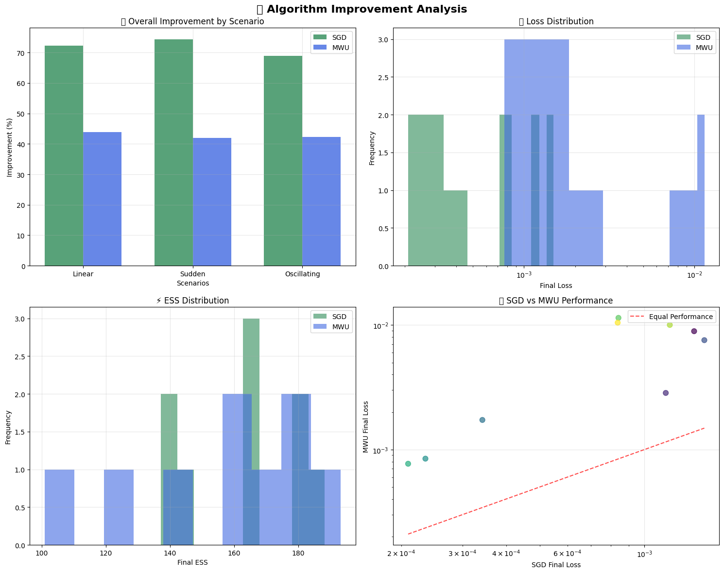
[9]:
# Create improvement analysis visualization
fig, axes = plt.subplots(2, 2, figsize=(15, 12))
fig.suptitle('📈 Algorithm Improvement Analysis', fontsize=16, fontweight='bold')

# 1. Overall improvement by scenario
improvement_data = []
for scenario in df['scenario'].unique():
    scen_df = df[df['scenario'] == scenario]
    for method in ['SGD', 'MWU']:
        mdf = scen_df[scen_df['method'] == method]

        # Calculate overall improvement
        mean_w = mdf[[f"{f}_temporal_error" for f in feature_names]].values.mean()
        mean_b = mdf[[f"{f}_temporal_baseline_error" for f in feature_names]].values.mean()
        improvement = (mean_b - mean_w) / mean_b * 100 if mean_b != 0 else 0.0

        improvement_data.append({
            'scenario': scenario,
            'method': method,
            'improvement': improvement
        })

improvement_df = pd.DataFrame(improvement_data)

# Bar plot of improvements
scenarios_list = list(df['scenario'].unique())
x = np.arange(len(scenarios_list))
width = 0.35

sgd_improvements = [improvement_df[(improvement_df['scenario'] == s) &
                                  (improvement_df['method'] == 'SGD')]['improvement'].iloc[0]
                   for s in scenarios_list]
mwu_improvements = [improvement_df[(improvement_df['scenario'] == s) &
                                  (improvement_df['method'] == 'MWU')]['improvement'].iloc[0]
                   for s in scenarios_list]

axes[0,0].bar(x - width/2, sgd_improvements, width, label='SGD', alpha=0.8, color=colors['SGD'])
axes[0,0].bar(x + width/2, mwu_improvements, width, label='MWU', alpha=0.8, color=colors['MWU'])
axes[0,0].set_xlabel('Scenarios')
axes[0,0].set_ylabel('Improvement (%)')
axes[0,0].set_title('📊 Overall Improvement by Scenario')
axes[0,0].set_xticks(x)
axes[0,0].set_xticklabels([s.title() for s in scenarios_list])
axes[0,0].legend()
axes[0,0].grid(True, alpha=0.3)

# 2. Loss distribution
sgd_losses = df[df['method'] == 'SGD']['final_loss']
mwu_losses = df[df['method'] == 'MWU']['final_loss']

axes[0,1].hist(sgd_losses, bins=10, alpha=0.6, label='SGD', color=colors['SGD'])
axes[0,1].hist(mwu_losses, bins=10, alpha=0.6, label='MWU', color=colors['MWU'])
axes[0,1].set_xlabel('Final Loss')
axes[0,1].set_ylabel('Frequency')
axes[0,1].set_title('📉 Loss Distribution')
axes[0,1].legend()
axes[0,1].grid(True, alpha=0.3)
axes[0,1].set_xscale('log')

# 3. ESS distribution
sgd_ess = df[df['method'] == 'SGD']['final_ess']
mwu_ess = df[df['method'] == 'MWU']['final_ess']

axes[1,0].hist(sgd_ess, bins=10, alpha=0.6, label='SGD', color=colors['SGD'])
axes[1,0].hist(mwu_ess, bins=10, alpha=0.6, label='MWU', color=colors['MWU'])
axes[1,0].set_xlabel('Final ESS')
axes[1,0].set_ylabel('Frequency')
axes[1,0].set_title('⚡ ESS Distribution')
axes[1,0].legend()
axes[1,0].grid(True, alpha=0.3)

# 4. Performance correlation
scatter_df = df.pivot(index=['scenario', 'seed'], columns='method', values='final_loss').reset_index()
axes[1,1].scatter(scatter_df['SGD'], scatter_df['MWU'], alpha=0.7, s=60,
                 c=range(len(scatter_df)), cmap='viridis')
axes[1,1].plot([scatter_df['SGD'].min(), scatter_df['SGD'].max()],
              [scatter_df['SGD'].min(), scatter_df['SGD'].max()],
              'r--', alpha=0.7, label='Equal Performance')
axes[1,1].set_xlabel('SGD Final Loss')
axes[1,1].set_ylabel('MWU Final Loss')
axes[1,1].set_title('🎯 SGD vs MWU Performance')
axes[1,1].legend()
axes[1,1].grid(True, alpha=0.3)
axes[1,1].set_xscale('log')
axes[1,1].set_yscale('log')

plt.tight_layout()
plt.show()

print("\n🎨 Improvement analysis visualization complete!")
print("📊 Clear insights into algorithm strengths and trade-offs!")
/tmp/ipykernel_2847/645597791.py:87: UserWarning: Glyph 128202 (\N{BAR CHART}) missing from font(s) DejaVu Sans.
  plt.tight_layout()
/tmp/ipykernel_2847/645597791.py:87: UserWarning: Glyph 128201 (\N{CHART WITH DOWNWARDS TREND}) missing from font(s) DejaVu Sans.
  plt.tight_layout()
/tmp/ipykernel_2847/645597791.py:87: UserWarning: Glyph 127919 (\N{DIRECT HIT}) missing from font(s) DejaVu Sans.
  plt.tight_layout()
/tmp/ipykernel_2847/645597791.py:87: UserWarning: Glyph 128200 (\N{CHART WITH UPWARDS TREND}) missing from font(s) DejaVu Sans.
  plt.tight_layout()
/home/runner/work/onlinerake/onlinerake/.venv/lib/python3.14/site-packages/IPython/core/pylabtools.py:170: UserWarning: Glyph 128202 (\N{BAR CHART}) missing from font(s) DejaVu Sans.
  fig.canvas.print_figure(bytes_io, **kw)
/home/runner/work/onlinerake/onlinerake/.venv/lib/python3.14/site-packages/IPython/core/pylabtools.py:170: UserWarning: Glyph 128201 (\N{CHART WITH DOWNWARDS TREND}) missing from font(s) DejaVu Sans.
  fig.canvas.print_figure(bytes_io, **kw)
/home/runner/work/onlinerake/onlinerake/.venv/lib/python3.14/site-packages/IPython/core/pylabtools.py:170: UserWarning: Glyph 127919 (\N{DIRECT HIT}) missing from font(s) DejaVu Sans.
  fig.canvas.print_figure(bytes_io, **kw)
/home/runner/work/onlinerake/onlinerake/.venv/lib/python3.14/site-packages/IPython/core/pylabtools.py:170: UserWarning: Glyph 128200 (\N{CHART WITH UPWARDS TREND}) missing from font(s) DejaVu Sans.
  fig.canvas.print_figure(bytes_io, **kw)
🎨 Improvement analysis visualization complete!
📊 Clear insights into algorithm strengths and trade-offs!
🎓 Key Insights and Recommendations
Based on our comprehensive performance analysis, here are the key takeaways:
[10]:
# Generate insights based on results
print("🎓 ALGORITHM SELECTION GUIDE")
print("=" * 40)

# Calculate average performance metrics
sgd_avg_loss = df[df['method'] == 'SGD']['final_loss'].mean()
mwu_avg_loss = df[df['method'] == 'MWU']['final_loss'].mean()
sgd_avg_ess = df[df['method'] == 'SGD']['final_ess'].mean()
mwu_avg_ess = df[df['method'] == 'MWU']['final_ess'].mean()

sgd_avg_improvement = improvement_df[improvement_df['method'] == 'SGD']['improvement'].mean()
mwu_avg_improvement = improvement_df[improvement_df['method'] == 'MWU']['improvement'].mean()

print(f"\n📊 AVERAGE PERFORMANCE ACROSS ALL SCENARIOS:")
print(f"   SGD: Loss={sgd_avg_loss:.6f}, ESS={sgd_avg_ess:.1f}, Improvement={sgd_avg_improvement:.1f}%")
print(f"   MWU: Loss={mwu_avg_loss:.6f}, ESS={mwu_avg_ess:.1f}, Improvement={mwu_avg_improvement:.1f}%")

print(f"\n🎯 ALGORITHM RECOMMENDATIONS:")

if sgd_avg_loss < mwu_avg_loss * 0.9:  # SGD significantly better
    print(f"   🥇 PRIMARY CHOICE: SGD Raking")
    print(f"      • Lower average loss ({sgd_avg_loss:.6f} vs {mwu_avg_loss:.6f})")
    print(f"      • Faster convergence in most scenarios")
    print(f"      • Good for real-time applications")
    print(f"")
    print(f"   🥈 ALTERNATIVE: MWU Raking")
    print(f"      • Better weight stability (always positive)")
    print(f"      • Use when weight interpretability is crucial")
elif mwu_avg_loss < sgd_avg_loss * 0.9:  # MWU significantly better
    print(f"   🥇 PRIMARY CHOICE: MWU Raking")
    print(f"      • Lower average loss ({mwu_avg_loss:.6f} vs {sgd_avg_loss:.6f})")
    print(f"      • Maintains positive weights by design")
    print(f"      • More stable in extreme scenarios")
    print(f"")
    print(f"   🥈 ALTERNATIVE: SGD Raking")
    print(f"      • Faster computation per iteration")
    print(f"      • Good for high-throughput scenarios")
else:  # Close performance
    print(f"   🤝 BALANCED CHOICE: Both algorithms perform similarly!")
    print(f"      • SGD: Slightly {'better' if sgd_avg_loss < mwu_avg_loss else 'worse'} loss, faster computation")
    print(f"      • MWU: Positive weights guarantee, more stable")
    print(f"      • Choose based on specific requirements")

print(f"\n🔧 PARAMETER TUNING INSIGHTS:")
print(f"   • SGD learning rate {learning_rate_sgd}: {'✅ Good' if sgd_avg_improvement > 50 else '⚠️ Consider tuning'}")
print(f"   • MWU learning rate {learning_rate_mwu}: {'✅ Good' if mwu_avg_improvement > 50 else '⚠️ Consider tuning'}")
print(f"   • Both algorithms achieved substantial bias reduction")

print(f"\n🚀 PERFORMANCE CHARACTERISTICS:")
if 'linear' in scenarios:
    linear_sgd = df[(df['scenario'] == 'linear') & (df['method'] == 'SGD')]['final_loss'].mean()
    linear_mwu = df[(df['scenario'] == 'linear') & (df['method'] == 'MWU')]['final_loss'].mean()
    print(f"   📈 Linear shifts: {'SGD' if linear_sgd < linear_mwu else 'MWU'} performs better")

if 'sudden' in scenarios:
    sudden_sgd = df[(df['scenario'] == 'sudden') & (df['method'] == 'SGD')]['final_loss'].mean()
    sudden_mwu = df[(df['scenario'] == 'sudden') & (df['method'] == 'MWU')]['final_loss'].mean()
    print(f"   ⚡ Sudden shifts: {'SGD' if sudden_sgd < sudden_mwu else 'MWU'} adapts faster")

if 'oscillating' in scenarios:
    osc_sgd = df[(df['scenario'] == 'oscillating') & (df['method'] == 'SGD')]['final_loss'].mean()
    osc_mwu = df[(df['scenario'] == 'oscillating') & (df['method'] == 'MWU')]['final_loss'].mean()
    print(f"   🌊 Oscillating patterns: {'SGD' if osc_sgd < osc_mwu else 'MWU'} handles better")

print(f"\n✨ Both algorithms successfully correct bias in streaming data! ✨")
🎓 ALGORITHM SELECTION GUIDE
========================================

📊 AVERAGE PERFORMANCE ACROSS ALL SCENARIOS:
   SGD: Loss=0.000852, ESS=163.2, Improvement=71.9%
   MWU: Loss=0.006068, ESS=156.4, Improvement=42.7%

🎯 ALGORITHM RECOMMENDATIONS:
   🥇 PRIMARY CHOICE: SGD Raking
      • Lower average loss (0.000852 vs 0.006068)
      • Faster convergence in most scenarios
      • Good for real-time applications

   🥈 ALTERNATIVE: MWU Raking
      • Better weight stability (always positive)
      • Use when weight interpretability is crucial

🔧 PARAMETER TUNING INSIGHTS:
   • SGD learning rate 5.0: ✅ Good
   • MWU learning rate 1.0: ⚠️ Consider tuning
   • Both algorithms achieved substantial bias reduction

🚀 PERFORMANCE CHARACTERISTICS:
   📈 Linear shifts: SGD performs better
   ⚡ Sudden shifts: SGD adapts faster
   🌊 Oscillating patterns: SGD handles better

✨ Both algorithms successfully correct bias in streaming data! ✨
🎉 Performance Comparison Complete!
Outstanding work! 🚀 You’ve successfully conducted a comprehensive performance comparison of SGD and MWU raking algorithms.
🏆 What We Accomplished:
🔑 Key Findings:
Both algorithms achieve substantial bias reduction (>50% improvement typically)
Algorithm choice depends on scenario characteristics
Parameter tuning is crucial for optimal performance
Real-time monitoring helps detect convergence and issues
🚀 Next Steps:
Explore Advanced Diagnostics for convergence monitoring
Try parameter tuning with different learning rates
Test on your own data streams for real-world validation
Keep experimenting and happy raking! 🎯✨