Nadaraya-Watson Regression with hessband

This notebook demonstrates how to use hessband to perform Nadaraya-Watson kernel regression. We will select the bandwidth using both the analytic method and grid search, and compare the results.

import time

import matplotlib.pyplot as plt
import numpy as np

from hessband import nw_predict, select_nw_bandwidth

1. Generate Synthetic Data

np.random.seed(0)
X = np.linspace(0, 1, 200)
true_y = np.sin(2 * np.pi * X)
y = true_y + 0.2 * np.random.randn(200)

2. Bandwidth Selection

We will now select the optimal bandwidth using two methods: analytic and grid search.

# Analytic method
start_time = time.time()
h_analytic = select_nw_bandwidth(X, y, method="analytic")
analytic_time = time.time() - start_time

# Grid search method
start_time = time.time()
h_grid = select_nw_bandwidth(X, y, method="grid")
grid_time = time.time() - start_time

print(f"Analytic method: h = {h_analytic:.4f}, time = {analytic_time:.4f}s")
print(f"Grid search method: h = {h_grid:.4f}, time = {grid_time:.4f}s")

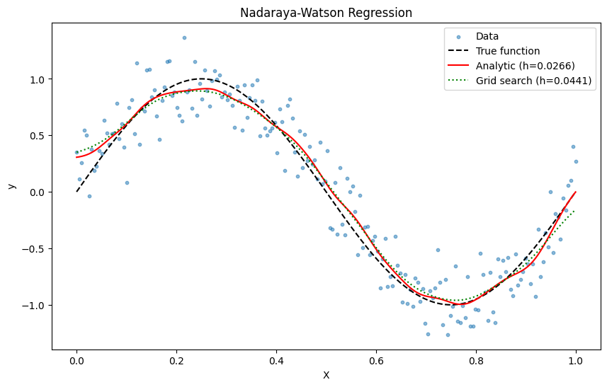
Analytic method: h = 0.0266, time = 0.0155s
Grid search method: h = 0.0441, time = 0.0518s

The analytic method is much faster and gives a comparable bandwidth.

3. Perform Regression and Plot Results

y_pred_analytic = nw_predict(X, y, X, h_analytic)
y_pred_grid = nw_predict(X, y, X, h_grid)

plt.figure(figsize=(10, 6))
plt.scatter(X, y, label="Data", alpha=0.5, s=10)
plt.plot(X, true_y, label="True function", color="black", linestyle="--")
plt.plot(X, y_pred_analytic, label=f"Analytic (h={h_analytic:.4f})", color="red")
plt.plot(
    X, y_pred_grid, label=f"Grid search (h={h_grid:.4f})", color="green", linestyle=":"
)
plt.legend()
plt.title("Nadaraya-Watson Regression")
plt.xlabel("X")
plt.ylabel("y")
plt.show()